Microchaos in human postural balance: Sensory dead zones and sampled time-delayed feedback

(1)

Microchaos in human postural balance: Sensory dead zones and sampled time-delayed feedback

John G. Milton,¹ Tamas Insperger,² Walter Cook,¹ David Money Harris,³ and Gabor Stepan⁴

1W. M. Keck Science Center, The Claremont Colleges, Claremont, CA 91711, USA

2Department of Applied Mechanics, Budapest University of Technology and Economics and MTA-BME Lend¨ulet Human Balancing Research Group, 1111 Budapest, Hungary

3Department of Engineering, Harvey Mudd College, Claremont, CA 91711

4Department of Applied Mechanics, Budapest University of Technology and Economics, 1111 Budapest, Hungary (Dated: July 20, 2018)

Models for the stabilization of an inverted pendulum figure prominently in studies of human balance control. Surprisingly, fluctuations in measures related to the vertical displacement angle for quietly standing adults with eye closed exhibit chaos. Here we show that small amplitude chaotic fluctuations (“microchaos”) can be generated by the interplay between three essential components of human neural balance control, namely, time-delayed feedback, a sensory dead zone and frequency- dependent encoding of force. When the sampling frequency of the force encoding is decreased, the sensitivity of the balance control to changes in the initial conditions increases. The sampled, time- delayed nature of the balance control may provide insights into why falls are more common in the very young and the elderly.

PACS numbers: 02.30.Ks, 07.05.Dz, 05.45.Ac

The identification of the mechanisms that stabilize unstable states is a relevant problem that receives increas- ing attention in physics, engineering, biology and neuroscience. A well studied paradigm involves the stabilization of an inverted pendulum using time-delayed feedback [1–3]. In particular, such models have been used to obtain insights into the neural control of balance and into how falls, a major cause of morbidity and mortal- ity in the elderly, might be prevented. An unexplained observation is that the fluctuations in measures related to the vertical displacement angle,θ, of quietly standing adults [4–7] and the movements of the trunk of a sitting infant [8] exhibit a positive maximum Lyapunov exponent (λ_max), namely a signature of a chaotic dynamical system [9, 10]. Chaotic dynamics can be controlled using time-delayed feedback [11]. However, little is known about how chaotic dynamics can arise in the context of the delayed feedback control of balance [12–14]. Thus an understanding of the mechanism that generates these low amplitude, chaotic fluctuations may provide important clues into the nature of human balance control [15].

Here we show that chaotic fluctuations can be generated by the interplay between three essential components of neural balance control, namely, time-delayed feedback, a sensory dead zone and the frequency-dependent encoding of force. A key observation is that the control forces for human balance control are exerted intermittently [17–

21]. Intermittency is suggestive of a sampled data system [22–24]. Two essential properties of a sampled data system are spatial quantization and temporal sampling [25].

In the context of neural balance control, temporal sampling arises because of spike frequency dependent neural force [26–28]. Spatial quantization of feedback arises because of the presence of sensory dead zones [29–32].

The combined effect of spatial quantization and temporal sampling produces an amplitude quantization because

the corrective forces are turned ON and OFF depending on whether the controlled variable is larger or smaller than a sensory threshold [32–34]. Time delays arise because of the time between when the nervous system de- tects an error and then acts upon it. Thus the chaotic fluctuations generated by balance control could arise in much the same way as occurs when digital time-delayed feedback is used to control a continuous-time Newtonian mechanical system in the presence of round-off error due to the finite precision numerical representation of the state variables (spatial quantization). Since the amplitude of these chaotic fluctuations are very small, the phenomenon is referred to as microchaos [12–14].

Our discussion is organized as follows. First we introduce the concept of a sampled, time-delayed data system through an analysis of a scalar delay differential equation.

Acting together spatial quantization due to the sensory dead zone (Section I) and temporal sampling due to frequency encoding (Section II) produces the low-amplitude chaos called microchaos. Finally in Section III we ex- tend our observations to an electronic implementation of delayed feedback control of an unstable fixed point and an experimentally validated model for the stabilization of human postural sway during quiet standing by time- delayed proportional-derivative (PD) feedback [2, 15, 16].

In all cases there is a sensitive dependence to the initial conditions for a range of sampling times.

I. QUANTIZED HAYES EQUATION

We illustrate the effects of amplitude quantization and time sampling (Section II) on the time-delayed feedback control of balance by considering the scalar delay differ-

(2)

ential equation (DDE)

˙

x(t) =x(t)−Gx(t−τ) (1) where τ is the time delay, G is the feedback gain and the ‘−’ before G indicates negative feedback (Fig. 1).

This equation, named the Hayes equation [35], frequently arises in the linear stability analysis of models for feedback control in engineering and biological applications [36–38]. In the context of balance control, (1) describes the control of an over-damped inverted pendulum, where θ is the angular position, x = `sinθ and ` is the distance of the center of mass from the contact point on the ground [33].

WhenG= 0, the fixed point x≡0 is unstable. The stability boundaries of (1) in the plane (G, τ) are given by the lineG= 1 and the parametric curve

G=p

ω²+ 1, τ= 1

ωatan(ω) (2)

withω∈[0,∞) (see red line in Fig. 1c).

The effect of quantization is that the feedback forces are computed using integer multiples of the quantization step,h. Hence (1) becomes the quantized Hayes equation

˙

x(t) =x(t)−GhInt

x(t−τ) h

, (3)

where Int() rounds towards zero. In contrast to (1), the stable solutions of (3) are limit cycle oscillations (Fig. 1b). Due to the piecewise constant forcing, the limit cycle oscillations can be determined by piecing together segments of exponential functions as

x(t) =









 . . .

2Gh+ (x0−2Gh)e^t−t⁰ if 2h≤x(t−τ)<3h, Gh+ (x0−Gh)e^t−t⁰ if h≤x(t−τ)<2h, x0e^t−t⁰ if −h < x(t−τ)< h,

−Gh+ (x0+Gh)e^t−t⁰ if −2h < x(t−τ)≤ −h,

−2Gh+ (x0+ 2Gh)e^t−t⁰ if −3h < x(t−τ)≤ −2h, . . .

wherex0=x(t0) andt0refers to the initial time instant of each segments. In other words, when x(t) crosses a threshold at timet=t_T, an integer change occurs in the feedbackτ later at instantt=t_T +τ. The amplitude of the oscillations scale withh[14]. Ifh→0 then (3) gives (1).

When

e^τ< G < e^τ

e^τ−1, (4)

there is a limit cycle oscillation bounded by either 0 <

x < 2h or by −2h < x < 0. The observed limit cycle depends on the choice of the initial condition. These solutions are confined to the region in (G, τ) designated S2. Whenτ <ln 2 and

e^τ

e^τ−1 < G < 3 +√

17−12e^τ+ 4e^2τ

2(e^τ−1) , (5)

0 1 2 3 4 5

0 0.2 0.4 0.6 0.8 1 1.2

-202

0 5 10 15 20 25 30

-202

0 1 2 3 4 5

0 0.2 0.4 0.6 0.8 1 1.2

-202

0 5 10 15 20 25 30

-202

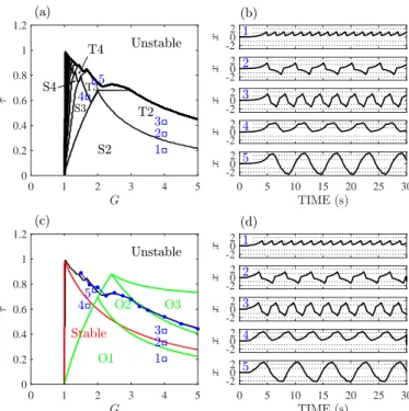
FIG. 1: Comparison of oscillatory solutions generated by (3) and by the electronic circuit described in Section III A. (a) Parameter regions for different types of bounded motions of (6) withR= 300). (b) Numerical simulations for parameter points 1-5 shown in a). (c) Boundaries of regions of bounded motions for the quantized-sampled Hayes equation (6) when R= 300 (black line) and for the circuit withR= 300 (blue dots). For comparison the red line give the stability region for the Hayes equation (1) and the green lines outline the parameter regions for the three different oscillatory solutions for the sampled Eurich-Milton equation (9). (d) Circuit output for parameter points 1-5 shown in c). In all cases the initial condition was the background noise in the analog part of the circuit, Vrms≈ 0.02 V. Whenh < Vrms the solution escapes from the basin of attraction.

then there exist solutions bounded in −2h < x < 2h.

This region is indicated by T2 in Figure 1a. Similarly, there exist regions, where the solutions are bounded in 0< x <3h, 0< x <4h, etc., indicated by S3, S4, etc., and in−3h < x <3h,−4h < x <4h, etc., indicated by T3, T4, etc. Examples of solutions for S2, T2 and S3, T3 are shown in Figure 1b.

II. QUANTIZED-SAMPLED HAYES EQUATION

The introduction of time discretization into the feedback requires the use of a time step ∆t such that τ = R∆t, where R is a positive integer. Hence (3) becomes the quantized-sampled Hayes equation

˙

x(t) =x(t)−GhInt

x(tj−R) h

, (6)

(3)

wheret∈[tj, tj+1) andtj=j∆t,j= 0,1,2. . . gives the time instants where the state variables are sampled. If

∆t→0 such thatR∆t→τ then (6) gives (3).

The sampling effect introduces a periodic parametric excitation in the time delay [40]. This can be seen by writingx(t_j−R),t∈[tj, tj+1) asx(t−ρ(t)) where

ρ(t) =R∆t+t−∆tInt t

∆t

, (7)

is a ∆t-periodic function. Thus (6) is equivalent to a time-periodic DDE (i.e. a DDE with time-periodic point delay) with principal period ∆t = τ /R. According to the Floquet theory [39], the stability conditions for linear time-periodic DDEs are determined by the eigenvalues of the monodromy operator, which for delayed systems is typically an infinite-dimensional operator. On the other hand (6) can also be considered as a system of ordinary differential equations with a piecewise constant forcing on the right hand side. The piecewise constant forcing arises when a zero order hold is applied over each time interval

∆t. Hence we have a finite-dimensional representation of the monodromy operator This is very similar to what occurs in a sampled data system [25]. These observations motivate the use of the semi-discretization method [40] to numerically integrate the DDEs with event-driven switching feedback considered in this communication.

Fig. 2 shows the effects of changingRon the dynamics generated by (6). As R decreases the solutions become increasingly sensitive to very small changes in the initial function (compare solid and dashed lines) (Fig. 2a). This is accompanied by a decrease in the number of harmonics in the power spectral density (Fig. 2c) and the enclosure of the orbits in the phase plane becomes larger (Fig. 2d).

The observations in Fig. 2 illustrate the phenomenon of microchaos (small-scale chaos). The key point is the realization that because of time sampling the switches in feedback do not typically occur when|x(t−τ)|=|h|, but rather when|x(t_j−R)| ≥ |h|and|x(t_j−R−1)|<|h|. This allows a fluctuation of the values ofx(t) at the switching instants within the range

|x(tj−R)−x(tj−R−1)| ≈ |he^R∆t−he^(R−1)∆t|

≤he^(R−1)∆t|(e^∆t−1)| ≈he^(R−1)∆t∆t. (8) Thus, depending on the value of R = τ /∆t, the fluctuations in x(t) can be so small that they may not be visually apparent (top panel in Fig. 2b). Even for large R, the solutions generated by two nearby choices of initial functions eventually separates. In other words, the rate of revolution of chaos is inversely proportional toR [41].

Collectively the observations in Figure 2 suggests a route from periodic motions to microchaos as R decreases. The sensitivity of the solutions to changes in the initial function suggest that the maximum Lyapunov exponent,λmax, is positive. This is not surprising. For small displacements, namely when|x(tj−R∆t)|< h, we

have exponential growth governed by ˙x(t) = x(t). Fig- ure 3 shows λmax calculated using the Wolf algorithm [10] as a function ofR. There is an inverse relationship betweenR andλ_max (see also Discussion).

The observations of microchaotic dynamics in Fig. 2 can also be mathematically supported by the fact that all of the solutions in Fig. 2 involve only crossings of thex=

±hthreshold. In this case the dynamics of the circuit are described by the sampled Eurich-Milton equation [33, 41]

˙

x(t) =x(t) +f(x(t_j−R)), (9) wheret∈[t_j, t_j+1) and

f(x(t_j−R∆t)) =







G if x(t_j−R)≤ −h, 0 if −h < x(t_j−R)< h,

−G if x(t_j−R)≥h .

(10) The green lines in Fig. 1c show the boundaries for the three types of limit cycle oscillations that exist as a function of (G, τ) [33, 41]. In the region of the parameter space where the solutions of the circuit correspond to solutions of (9), it has been proven that the dynamics are chaotic whenR= 0 [41].

III. APPLICATIONS

We anticipate that the addition of a sensory dead zone and sampling to models for the stabilization of an unstable state, such as that possessed by an inverted pendulum, will result in a sensitivity to initial conditions for a range of ∆t. Here we present two examples for which this conjecture is true.

A. Digital feedback control

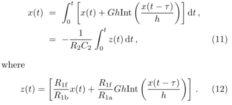
Digital feedback controllers are ubiquitous in atomic, molecular and optical physics [44, 45], where, for exam- ple, it has been possible to use this technique to control the trajectory of a single atom [46] and to explore entropy production in a photon-counting optoelectrnic feedback oscillator [47]. Time delays and the limitations of sensors are important considerations. Equation (6) can be implemented as the electronic circuit shown in Fig. 4 (see Appendix). Briefly

x(t) = Z t

0

x(t) +GhInt

x(t−τ) h

dt ,

= − 1

R2C2

Z t 0

z(t) dt , (11)

where z(t) =

R1f

R1b

x(t) + R1f

R1a

GhInt

x(t−τ) h

. (12)

(4)

0 10 20 30 -2

-1 0 1 2

0 10 20 30

1.49 1.492 1.494

0 2 4 6

-150 -100 -50 0 50

-2 -1 0 1 2

0 10 20 30

-2 -1 0 1 2

0 10 20 30

1.4 1.45 1.5 1.55 1.6

0 2 4 6

-150 -100 -50 0 50

-2 -1 0 1 2

0 10 20 30

-2 -1 0 1 2

0 10 20 30

1.4 1.5 1.6 1.7

0 2 4 6

-150 -100 -50 0 50

-2 -1 0 1 2

FIG. 2: Sensitivity of the dynamics of (6) to different initial functionsx(ϑ) ≡0.5 and 0.6 forϑ∈[−τ,0] when G= 4.0 and τ = 0.438 s. a) Solutions for two nearby choices of the initial condition are shown (solid and dashed black red line) for three values ofR. b) Maxima of solution in (a) at zoomed scale to demonstrate microchaotic fluctuations. c) Power spectral densities (PSD) and d) phase plane projections for the three values ofRshown in a).

0 50 100 150 200 250 300

0 0.2 0.4 0.6 0.8

FIG. 3: Maximal Lyapunov exponent as function of R for numerical simulations of (4). Maximal Lyapunov exponent was determined using the numerical method described in [10] using Wolf’s Matlab program downloaded from Matlab central.

[10].

The values of resistorsR2, R1a, R1b, R1f and capacitor C2are given in Fig. 4. The first term of the integral is the solution of the continuous dynamical system ˙x(t) =x(t).

This part of the circuit is implemented using operational amplifiers. The second term of the integral represents the effects of time-delayed digital negative feedback and was constructed using a microprocessor (Arduino Mega, sampling frequency 1000 Hz). This microprocessor was programmed to quantize the feedback and to introduce the time delay using a circular buffer. The input to the microprocessor was low-pass filtered (LPF) in order to minimize the effects of high frequency noise on the timing of threshold crossings. It is understood from (6) that for

FIG. 4: Schematic representation of the electronic circuit used to model (3) and (6). The circuit is manually triggered by briefly closing the reset switch then typically inputting a square wave pulse of durationτ by holding the switch at IC.

It is also possible to trigger the circuit by briefly closing the reset switch and IC, then allowing the internal noise in the circuit to autotrigger the oscillator. See also the Appendix and Supplementary Material [48].

each time interval of length ∆tthe force generated by the digital feedback is kept constant, namely there is a zero- order hold approximation. The sample-and-hold (S/H)

(5)

0 50 100 150 200 250 300 0

0.5 1 1.5 2 2.5

0 5 10 15 20

-2 0 2

0 5 10 15 20

-2 0 2

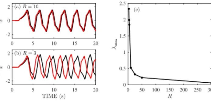
FIG. 5: Dynamics of the circuit shown in Fig. 4. (a) and (b) show the time series obtained for two initial conditions due to different background noise (about Vrms ≈ 0.26 and 0.32 for R=10 and 0.26 and 0.33, respectively, for R=3) (red and black) for two different values ofRwhenτ= 0.425s and G= 4.0). (c)λmaxas a function ofR.

circuit (1 % duty cycle) enables the feedback forces to be sampled at a lower frequency than the circuit sampling frequency.

Qualitatively similar solutions are observed in the circuit as for numerical simulations of (6) for the same choices of G and τ (compare Fig. 1b and d). How- ever, since the circuit contains capacitance, the switches in feedback do not occur instantaneously as in (6), but there is a small, but finite rise time and fall time. This may explain why the the circuit appears to have a greater sensitivity to change in the initial conditions and hence for a givenR there is a largerλmax(Fig. 5).

B. Postural sway

Human balance during quiet standing is often modeled by a second-order delay differential equation of the form [2, 15, 16, 49–51]

θ(t)¨ −ω²_nθ(t) =T(t−τ) (13) whereωnis the characteristic frequency of the system,τ is the time delay (≈ 0.1s [16, 52]) and T is the restor- ing torque. Following the parameters in [15], ω²_n = (M gH−K_pass)/J, where M = 60kg is the mass of the body without the feet,g= 9.81m/s² is the gravitational acceleration,H = 1m is the distance between the center of mass and the ankle joint,Kpass= 0.8M gH is the pas- sive stiffness of the ankle and J = 60kgm² is the mass moment of inertia with respect to the ankle joint. These parameters giveω_n= 1.4s⁻¹.

The principal sensory input during quiet standing with eye closed is from proprioceptive sensors in the ankle joint [29, 53], namely the Golgi tendon organs and muscle spindles [30]. Under these conditions the functional form for T becomes

T(t) =Tp(t) +Td(t), (14)

0 5 10 15 20

0 0.1 0.2 0.3 0.4 0.5

0 5 10 15 20

-0.5 0 0.5

0 5 10 15 20

-0.5 0 0.5

FIG. 6: Dynamics of the PR model of postural sway described by (13)-(14). (a) and (b) show the time series obtained for two initial conditions,θ(0) = 0.1 deg and 0.12 deg (red and black) for two different values ofR. (c)λmaxas a function of Rforτ= 0.1s(solid line) andτ= 0.125s(dashed line).

where T_p(t) =

(0 if|θ(tj−R)|< Πpos

−k_pθ(t_j−R) if|θ(t_j−R)| ≥Π_pos, (15) T_d(t) =

(0 if|θ(t˙ _j−R)|< Π_vel

−kdθ(t˙ _j−R) if|θ(t˙ _j−R)| ≥Πvel, (16) with t ∈ [t_j, t_j+1), t_j = j∆t, and k_p = 20s⁻² and kd= 4s⁻¹ are, respectively, the proportional and derivative gains. The sensory dead zone for the body’s angular position,Πpos, is 0.1 deg. This value has been estimated using small mechanical ankle displacements [29] and from the two-point correlation function [31]. The dead zone for the angular velocity,Π_velwas assumed to be 1 deg/s. For these parameters the oscillations in the postural away angle are of the order of 0.5 deg as observed experimentally [54].

Figure 6 shows the sensitivity of the solutions of (13)- (14) to initial conditions. As observed for the quantized- sample Hayes equations and its electronic implementation, λmax becomes more and more positive as R decreases. The spike frequencies recorded for muscle spindles and Golgi tendon organs suggest that ∆t ≈ 0.005−0.03s [55, 56]. For this range of ∆t we obtain λmax≈0.02−0.2 (see Fig. 6c). If the electro-mechanical delay is included, τ become 0.125s ([51] and the value of λmax changes as a function of R (see dashed line in Fig. 6c.

Estimates ofλ_maxpostural sway during quiet standing with eye closed range from<0 [58, 59], to 0.063 [6], 0.1 [15], 0.2-0.5 [7] and 1.9 [5]. The observations in Fig. 6 are consistent with estimates ofλmax≤0.2.

IV. DISCUSSION

Our mechanism for producing microchaos can be read- ily understood intuitively. In mathematical models the three sufficient conditions for chaos are well established

(6)

[57]: sensitivity to initial conditions, the existence of closed invariant sets, and mixing. For small x, namely, when|x(tj−R∆t)|< h, we have ˙x(t) =x(t) and hence the Lyapunov exponent is positive. Thus there is a sensitivity to initial conditions. The negative feedback ensures that invariant sets exist for appropriate choices ofGand τ. Finally, the limit cycle dynamics together with the effects of time discretization on determining threshold crossings provide a mechanism for mixing. These intu- itions have been established analytically for some sim- plified versions of (6) [12, 41]. Although it has been suggested that a positiveλmax for postural sway can be generated by weakly perturbing an intermittent control mechanism with a low amplitude periodic input [15], our observations suggest that microchaos can be an intrinsic component of the control mechanism.

Our main observation is that a quantized, time- sampled DDE model for balance control is capable of reproducing the positiveλ_maxvalues measured by exper- imentalists for human postural sway using the Wolf algorithm. In general the Wolf algorithm is not well suited for estimating λmax for chaotic DDEs. The fundamen- tal problem is that such dynamical systems are infinite dimensional. In contrast, the quantized, time-sampled DDE model we propose for human balance control is finite dimensional. In fact, our model is equivalent to a (R+ 1)-dimensional system of ODEs. Thus we anticipate that the Wolf algorithm would be capable of, at least, reliably detecting the sign of λmax. Indeed, the Wolf algorithm obtains a positive λ_max for (9) when R = 0 as predicted [41]. However, the accuracy ofλ_max determined by the Wolf algorithm is not known. The ongoing development of more powerful methods for measuring the spectrum of Lyapunov exponents for DDEs [42, 43] may enable quantitative comparisons to be made between the predicted and measured values ofλ_max.

Our observations demonstrate that chaotic dynamics can be robustly generated by a time-delayed intermittent control strategy in which there is frequency-dependent force encoding. We assumed that the changes in the feedback force are small and hence ∆t is constant. The microchaotic fluctuations have no effect on large scale stability, but provide evidence for the existence of an intermittent control strategy and the presence of a frequency dependent encoding of muscle force. It is not difficult to imagine that there may be situations when it is important to consider that ∆t changes. This would result is a novel dynamical system in which there is a state-dependent delay related to force.

The implication of our observations is that in dynamical systems with event-driven intermittent control there exists a direct link between the maximum positive Lya- punov exponent,λmax, signal quantization and the sampling frequency of time-delayed feedback. Quantization of visuomotor tasks is observed in the movements of the very young and older adults with disorders of the nervous system [60–62]. The demonstration that sampled data systems are also involved in human balance control

is expected to provide insights into why balance control often fails in the very young and the elderly.

ACKNOWLEDGMENTS

We acknowledge Edgar Perez (Reed College) for help- ful discussions. The research has received funding from the European Research Council under the European Unions Seventh Framework Program (FP7/2007-2013) / ERC Advanced grant agreement No340889 (SG,IT) and from the William R Kenan, Jr Charitable trust (JM).

The research reported in this paper was supported by the Higher Education Excellence Program of the Min- istry of Human Capacities in the frame of Biotechnology research area of Budapest University of Technology and Economics (BME FIKP-BIO).

APPENDIX

Details necessary to construct the circuit shown in Fig. 4 are given in the Supplementary materials. Here we describe the salient features of this circuit.

The electronic circuit consists of an unstable oscillator that is wired into a feedback loop with a programmed Ar- duino MEGA board. The oscillator is constructed with operational amplifiers and consists of a 2-stage unstable amplifier with an inverting pre-amp and inverting inte- grator. The Arduino board is programmed to provide three functions. First it converts the instantaneous analog waveform voltage from the oscillator at 1000Hz and reads them into a circular delay buffer that delays the feedback signal to the oscillator by an amount τ. Sec- ond, the input signal to the Arduino board is quantized by level detecting voltages above a set voltage. When the quantization level is less than 0.005V we refer to the feedback as“continuous”. When the quantization level is greater than 0.005V the feedback is referred to as “quantized”. Third, the polarity of the input is inverted to produce negative feedback. Finally, the feedback signal amplitude is multiplied by the feedback gain, G, using an adjustable gain, non-inverting amplifier on the circuit board.

The input waveform to the Arduino is the rectified (see below) unstable amplifier response signal and the recov- ered low-pass filter output of the Arduino is the quantized negative feedback signal. These two signals have entirely different shapes. The input and output signals of the Arduino require special attention.

The analog input to the Arduino A to D converter (ADC) (input A0) must be a positive voltage. However, the signal generated by the remainder of the circuit can be positive or negative. This problem cannot be sim- ply overcome by offsetting the signal, namely adding a constant positive voltage before the signal is inputted to the Arduino board and then adding a constant negative

(7)

voltage to the output to re-establish the negative feedback. This level shifting procedure does not solve the requirement that Int(x) is 0 when x is between −1 and +1. Although it is possible to overcome the problem in software we elected to solve it in hardware by construct- ing a precision op amp full-wave rectifier at the Arduino A0 input. The rectifier directly passes positive signal al- terations to A0 while inverting negative alternations and rectifies even millivolt level signals. Consequently the Arduino inputs to A0 are always positive.

The analog output of the Arduino is pulse width mod- ulated (PMW) and consists of 0 to +5V variable duty-

cycle pulses. This PWM output signal is then syn- chronously demodulated and low-pass filtered to recover both the positive and negative signal feedback waveform.

The linear range of the circuit was estimated as follows: When the response signal amplitude increased above 2V peak voltage we observed that the abrupt exponential segments of the waveform gradually appeared more rounded and continuous (see Fig. 1) until it be- came nearly sinusoidal when it reached 4V peak voltage.

Based on these observations we took the linear range of the circuit to be -2.5V to + 2.5V.

[1] J. Milton, J. L. Cabrera, T. Ohira, S. Tajima, Y.

Tonosaki, C. W. Eurich and S. A. Campbell, Chaos 19, 026110 (2009).

[2] G. Stepan, Philos. Trans. A Math. Phys. Eng. Sci.367, 1195 (2009).

[3] T. Insperger and J. Milton, Biol. Cybern.108, 85 (2014).

[4] N. Yamada, Hum. Mov. Sci.14, 711 (1995).

[5] S. F. Donker, M. Roerdink, A. J. Greven and P. J. Beek, Exp. Brain Res.181, 1 (2007).

[6] L. Ladislao and S. Fioretti, Med. Biol. Eng. Comput.45, 679 (2007).

[7] K. Liu, H. Wang, J. Xiao and Z. Taha. Comput. Intell.

Neurosci.2015, 158478 (2015).

[8] J. E. Deffeyes, R. T. Harbourne, A. Kyvelidou, W. A.

Stuberg and N. Stergiou, Clin. Biomech.24, 564 (2009).

[9] M. T. Rosenstein, J. J. Collins and C. J. DeLuca, Physica D65, 117 (1993).

[10] A. Wolf, J. B.Swift, H. L. Swinney and J. A. Vastano, Physica D16, 285 (1985).

[11] K. Pyragas, Phys. Lett. A170, 421 (1992).

[12] G. Haller and G. Stepan, J. Nonlin. Sci6, 415 (1996).

[13] E. Enikov and G. Stepan, J. Vib. Control2, 427 (1998).

[14] G. Stepan, J. Milton and T. Insperger, Chaos27, 114306 (2017).

[15] T. Nomura, S. Oshikawa, Y. Suzuki, K. Kiyono and P.

Morasso, Math. Biosci.245, 86 (2013).

[16] J. H. Pasma, T. A. Boonstra, J. van Kordelaar, V. V.

Spyropoulou and A. C. Schouten, Front. Comput. Neu- rosci.11, 99 (2017).

[17] J. L. Cabrera and J. G. Milton, Phys. Rev. Lett. 89, 158702 (2002).

[18] I. D. Loram and M. Lakie, J. Physiol.540, 1111 (2002).

[19] I. D. Loram, C. N. Maganaris and M. Lakie, J. Physiol.

564, 281 (2005).

[20] I. D. Loram, C. N. Maganaris and M. Lakie, J. Physiol.

564, 295 (2005).

[21] H. Tanabe, K. Fujii and M. Kouzali, Sci. Rep.7, 10631 (2017).

[22] P. J. Gawthrop, Proc. Inst. Mech. Eng. I J. Syst. Control Eng.223, 591 (2009).

[23] P. J. Gawthrop, I. Loram, M. Lakie and H. Gollee, Biol.

Cybern. 104, 31 (2011).

[24] I. D. Loram, H. Gollee, M. Lakie and P. J. Gawthrop, J.

Physiol.589, 307 (2011).

[25] T. Chen and B. A. Francis,Optimal sampled-date control systems(Springer-Verlag, New York, 1995).

[26] E. D. Adrian and Y. Zotterman, J. Physiol. 61, 151 (1926).

[27] L. R. Wilson, S. C. Gandevia, J. T. Inglis, J.-M. Gracies and D. Burke, Brain122, 2079 (1999).

[28] J. Day, L. R. Bent, I. Birznieks, V. G. Macefield and A.

G. Cresswell, J. Neurophysiol.117, 1489 (2017).

[29] R. Fitzpatrick and D. I. McCloskey, J Physiol.478, 173 (1994).

[30] I. D. Loram, M. Lakie, I. Di Guilo and C. N. Maganaris, J. Neurophysiol.102, 460 (2009).

[31] J. Milton, T. Insperger and G. Stepan in Mathemati- cal approaches to biological systems: Networks, oscilla- tors and collective phenomena, edited by T. Ohira and T. Ozawa (Springer, New York, 2015), pp. 1-15.

[32] J. Milton, R. Meyer, M. Zhvanetsky, S. Ridge and T.

Insperger, J. R. Soc. Interface13, 20160212 (2016).

[33] C. W. Eurich and J. G. Milton, Phys. Rev. E54, 6681 (1996).

[34] P. Kowalcyzk, P. Glendinning, M. Brown, G. Medraro- Cerda, H. Dallali and J. Shapiro, J. R. Soc. Interface9, 234 (2009).

[35] N. D. Hayes, J. London Math. Soc.25, 226 (1950).

[36] L. Glass and M. C. Mackey,From Clocks to chaos: The rhythms of life, (Princeton University Press, New Jersey, 1988).

[37] T. Erneux,Applied delay differential equations(Springer, New York, 2009).

[38] H. L. Smith,An introduction to delay differential equations with applications to the life sciences(Springer, New York, 2010).

[39] J. K. Hale and S. M. V. Lunel,Introduction to Functional Differential Equations, (Springer, New York, 1993).

[40] T. Insperger and G. St´ep´an,Semi-discretization for time- delay systems: Stability and engineering applications (Springer, New York, 2011).

[41] T. Insperger, J. Milton and G. Stepan, SIAM J. Appl.

Dyn. Sys.14, 1258 (2015).

[42] D. Breda and E. V. Vleck, Numer. Math. 126, 225 (2014).

[43] D. Breda and S. D. Schiava, Discrete Continuous Dyn.

Syst. Ser. B23, 2727 (2018).

[44] J. Bechhoefer, Rev. Mod. Phys.77, 783 (2005).

[45] D. R. Leibrandt and J. Heidecker, Rev. Sci. Instrum.86, 123115 (2015).

[46] A. Kubanek, M. Koch, C. Sames, A. Ourjoumtsev, P. W.

Pinske, M. Murr and G. Rempe, Nature462, 898 (2009).

(8)

[47] A. M. Hagerstrom, T. E. Murphy and R. Roy, Proc. Natl.

Acad. Sci. USA112, 9258 (2015).

[48] See Supplementary Material at [] for additional details concerning construction of circuit, Arduino code and the circuit diagram.

[49] C. Maurer and R. Peterka, J. Neurophysiol. 93: 189 (2005).

[50] T. Kiemel, K. S. Oie and J. J. Jeka, J. Neurophysiol.95, 1410 (2006).

[51] Y. Li, W. S. Levine and G. E. Loeb, IEEE Trans. Neural Syst. Rehabil. Eng.20, 738 (2012).

[52] M. H. Woollacott, C. von Hosten and B. R¨osbald, Exp.

Brain Res.72, 593 (1988).

[53] I. K. Wiesmeier, D. Dalin and C. Maurer, Front. Aging Neurosci.7, 97 (2015).

[54] J. Milton, J. Gyorffy, J. L. Cabrera and T. Ohira. US- NCTAN 2010-791 (2010).

[55] R. D. Pollock, R. C. Woledge, F. C. Maryin and D. J.

Newham, J. Appl. Physiol.112, 388 (1985).

[56] G. Macefield, K. Hagbarth, R. Gorman, S. C. Gandevia and D. Burke, J. Physiol.440, 497 (1991)

[57] S. Wiggins, Chaotic Transport in Dynamical Systems (Springer-Verlag, New York, 1992).

[58] J. J. Collins and C. J. De Luca, Phys. Rev. Lett.73, 764 (1994).

[59] P. Pascolo, F. Barazza and P. Carniel (2006). Chaos Soli- tons Fractals27, 1339 (2006).

[60] T. E. Milner and M. M. Ijaz, Neuroscience 35, 365 (1990).

[61] C. von Hofsten, J. Mot. Behav.23, 280 (1991).

[62] H. I. Krebs, M. L. Aisen, B. T. Volpe and N. Hogan, Proc. Natl. Acad. Sci. USA96, 4645 (1999).