Co-Exceedances in Eurozone Sovereign Bond Markets: Was There a Contagion during the Global Financial Crisis and the Eurozone Debt Crisis?

Co-Exceedances in Eurozone Sovereign Bond Markets: Was There a Contagion during the Global Financial Crisis and the Eurozone Debt Crisis?

Silvo Dajčman

University of Maribor, Faculty of Economics and Business, Razlagova 14, 2000 Maribor, Slovenia, e-mail silvo.dajcman@uni-mb.si

Abstract: The paper examines contagion between the sovereign bond markets of six Eurozone countries (France, Germany, Ireland, Italy, Spain, and Portugal) in the period from January 2000 to August 2011. A multinomial logistic model is applied to analyze contagion based on measuring joint occurrences of large yield changes (i.e., co- exceedances), while controlling for developments in common and regional factors that affect all sovereign bond markets simultaneously. I found that the Eurozone’s stock markets (EUROSTOXX50) returns, United States’ Treasury note yields, and the Euro-U.S. dollar (EUR-USD) exchange rate significantly impact the probability of extreme positive yield moves in the Eurozone’s sovereign bond markets. Positive EUROSTOXX50 returns and upside moves in U.S. Treasury note yields increased the probability of extreme positive sovereign bond yield moves in the Eurozone, whereas an increase in the EUR-USD exchange rate significantly reduced the probability. Conditional volatility in the Eurozone stock markets and the money market interest rate do not significantly impact the probability of extreme yield increases in the Eurozone’s sovereign bond markets. Furthermore, the probability of observing exceedance across Eurozone sovereign bond markets increased dramatically during the Eurozone debt crisis compared to the pre-crisis period. This study’s results also indicate less synchronous extreme yield dynamics across the Eurozone sovereign bond markets during the global financial crisis, especially during the Eurozone debt crisis compared to the pre-crisis period.

Keywords: Sovereign bond markets; Eurozone debt crisis; Contagion

1 Introduction

In recent years, European countries have been hit by two episodes of major financial market distress: the global financial crisis and the sovereign debt crisis.

The Eurozone sovereign debt crisis, triggered by mounting concerns about the fiscal sustainability of Mediterranean countries, led to a further surge in sovereign

bond yields. The shock spilled over to other Eurozone sovereign debt markets, thereby raising the question whether public debts across the Eurozone are sustainable. Prompted by financial market pressures, large-scale fiscal austerity measures have been announced in practically all Eurozone countries and sovereign debt management has advanced to the top of the international policy agenda.

As [16] argued, quantifying the exposure of developed countries to sovereign bond market spillovers (i.e., exposure to contagion) can help policymakers gain insight into overall financing constraints, as well as the external risks an economy faces. By analyzing contagion, knowledge is gained regarding whether a shock in one segment of a national financial market is transmitted across markets via channels that appear only during turbulent periods, or whether these shocks are transmitted via channels or inter-linkages that exist in all states of the world (non- crisis or crisis periods). [11] noted that the effectiveness of economic policy measures aimed at reducing a market’s vulnerability to contagion will depend on whether the contagion occurred as a result of the transmission of shocks through pre-existing, long-term links or through crisis contingent channels.

The literature includes many definitions of contagion (see e.g. [2], [4], [5], [9], [18]). [9] provides one of the most commonly accepted definitions of contagion, namely the “shift contagion”, which regards contagion as a shift or change in how shocks spread from one country (or asset class) to another during normal periods (pre-crisis) and how during crisis periods.¹ A common way to measure contagion is through the conditional correlation changes between the returns of asset classes.

Using this approach, contagion is identified if conditional correlation significantly increases in the crisis period in relation to the tranquil (non-crisis) periods. This method has been applied both empirically and extensively (e.g. by [4], [10]).

Correlations that give equal weight to small and large returns, however, are not appropriate to evaluate the differential impact of large returns (or yields in the case of bonds). As [1] argued, when large shocks exceed some threshold they can generate panic and propagate across countries. This propagation, however, is hidden in correlation measures by the large number of days when little of importance happens. Furthermore, the correlation coefficient is not an adequate measure of co-movement or interdependence and is difficult to interpret due to its sensitivity to heteroskedasticity (see [14] and [10]). The correlation coefficient is also a linear measure that is inappropriate if contagion is not a linear phenomenon but rather an event characterized by nonlinear changes in market associations [1].

1 Contagion must be distinguished from interdependence. As [10] argued, if two markets are traditionally highly correlated, and the correlation does not increase significantly after a shock in one market, then any continued high level of market co- movement suggests strong and real linkages between the two economies. In this case, there is no contagion but only high interdependence.

Rather than computing correlations of bond yield changes, here I base the analysis of contagion in sovereign bond markets on a measure of the joint occurrences of large positive yield changes (i.e., co-exceedances), an extreme value theory concept that [1] introduced. Exceedance is defined as an occurrence of a large bond yield change, that is, one above a certain threshold. Co-exceedances, on the other hand, are joint exceedances of two financial market returns above a certain threshold. This measure circumvents problems associated with the correlation coefficient because co-exceedances are not biased in periods of high volatility and are not restricted to modeling linear phenomena (see [3] and [6]).

A multinomial logistic regression can be used to model the occurrences of large bond yield changes. An important advantage of multinomial logistic analysis is that one can condition on attributes and characteristics of the exceedance events using control variables (or covariates) measured with information available up to the previous day. Following [1], the strength of contagion between sovereign bond markets is then measured as the fraction of co-exceedance of extreme positive bond yield changes that are not explained by the covariates included in the model.

In the present paper, I use a method developed by [1] to measure the strength of contagion between the sovereign bond markets of six Eurozone countries (France, Germany, Ireland, Italy, Spain, and Portugal) in the period from January 2000 to August 2011. A multinomial logistic model is applied to measure contagion between sovereign bond markets in a pair-wise manner. In other words, contagion is measured between pair-wise observed sovereign bond markets. To separate contagion from interdependence, I include more covariates in the multinomial logistic model than did [1] following suggestions in the empirical literature on contagion in the financial markets ([6], [7]). This includes the average stock market returns of the Eurozone (proxied by the returns on the EUROSTOXX50 index); the conditional volatility of the EUROSTOXX50 returns modeled as EGARCH(1,1); Eurozone money market interest rate level (3-month EURIBOR);

U.S. Treasury note yield changes; and returns on the Euro-U.S. dollar (EUR-USD) exchange rate. The response of probability estimates to the full range of values associated with different covariates are also computed and presented graphically to inspect whether the relationship between the probability of (co-)exceedances and covariates are linear or nonlinear. A multinomial logit model is specified in a way that enables us to investigate whether the most recent episodes of financial market distress (i.e., the global financial crisis and the Eurozone debt crisis) significantly impacted the probability of contagion in the investigated Eurozone sovereign bond markets.

2 Methodology

Exceedances in terms of extreme positive sovereign yield changes in a particular country and pair-wise joint occurrence (i.e., joint occurrence in two observed sovereign bond markets or co-exceedance) of extreme positive sovereign bond yield changes can be modeled as a polytomous variable. The dependent polytomous variable at time ( ; ) in the present paper can fall into one of three categories ( ): no exceedance in any of the pair-wise countries ( ); exceedance observed in one of the countries in the pair ( );

and co-exceedance. This third category represents a simultaneous exceedance in both the countries, representing contagion ( ). Probabilities associated with the events captured in the polytomous variables can then be estimated using a multinomial logistic model ([1]). An advantage of multinomial logistic analysis is that one can condition on attributes and characteristics of the exceedance events using control variables (explanatory variables or covariates) that are measured using information available up to the previous day.

The multinomial logit model assumes that the probability of observing category (of the three possible categories) in the dependent polytomous variable, , is given by Equation (1) ([11])

( ) _∑ ⁽ ₍ ⁾ ₎

, (1)

where is a matrix of covariates (with being the number of different covariates) and the vector of coefficients (including a constant) of a particular category associated with the covariates.² The covariates included in the model are the average stock market returns of the Eurozone (proxied by returns on the EUROSTOXX50 index); the conditional volatility of the EUROSTOXX50 returns modeled as EGARCH(1,1)³; the Eurozone money market interest rate level (3- month EURIBOR); 10-year U.S. Treasury note yield changes; and returns on the EUR-USD exchange rate. Because I also want to answer the question of whether the probability of contagion increases in a crisis period compared to a non-crisis period, also two dummy variables are included.⁴ The first dummy variable

2 To separate contagion from interdependence, it is important to identify common and regional factors that impact all countries simultaneously ([6]). A failure to model common and regional factors may result in tests of contagion being biased toward a positive finding of contagion.

3 The EGARCH model of [16] stipulates that negative and positive returns have different impacts on volatility.

4 Changes in Treasury note yields and the EUR-USD exchange rate (log) returns are included as a proxy for global macroeconomic developments and the associated inflation, liquidity, and credit risks (see e.g. [10] and [6]; [16]). The region-specific factors that capture local financial market conditions are the Eurozone money market rate, EUROSTOXX50 index, and its conditional volatility. As argued by [7], the bond markets should not be studied in isolation, because there are interaction effects across

represents the crisis period from September 16, 2008⁵ to April 22, 2010 and the second represents the crisis period from April 23, 2010 to August 31, 2011⁶. Coefficients are specific to each category, so that there are coefficients to be estimated. The coefficients are not all identified unless one imposes a normalization (see [12]). Normalization in the present paper is achieved by setting the coefficient of the first category ( ) to be zero. All regression coefficients of Equation (1) are thus calculated with respect to the first category (category 1) as a base category.

The model is estimated using maximum likelihood with the log-likelihood function for a sample of observations given by

∑ ∑ ( ), (2) where is a dummy variable that takes a value one if observation takes the th category and zero otherwise. Because is a nonlinear function of the , an iterative Newton-Rahpson’s estimation procedure is applied. Goodness-of-fit is measured using the pseudo- of [15] where both unrestricted (full model) likelihood, , and restricted (constants only) likelihood, , functions are compared

( ). (3)

After calculating regression coefficients, the probabilities of each of the three categories, , are computed by evaluating the covariates at their unconditional values

( )

∑ ( ), (4)

where is the vector of the unconditional mean values of the covariates. Because the coefficients in a multinomial logit model are difficult to interpret, following [12] and [1], the marginal changes in probability for a given unit change in the independent covariate (i.e., marginal effects) are calculated and tested whether they are significantly different from zero. The marginal effects ( ) are given by the following equation (see [12]):

|

[ ∑ ]| . (5)

different asset classes. In their study, [1] included only conditional volatility of the stock market, exchange rate returns, and the interest rate level.

5 On September 16, 2008 the investment bank Lehman Brothers collapsed and started the global financial crisis.

6 On April 23, the Greek government requested a bailout from the EU/IMF. I take this date as the start of the sovereign debt crisis in the Eurozone. August 31, 2011 is the end of the observation period in the paper.

[1] noted that it is often difficult to judge whether changes in probabilities of a given category are economically large or small. In the present paper, therefore, I also present the responses of probability estimates to the full range of values associated with different covariates, rather than just at its unconditional means, and present them graphically.

3 Data and Empirical Results

Extreme upper tail yield behavior in the sovereign bond markets in the six Eurozone countries, listed in Table 1, is analyzed based on the sovereign bond yield changes. The daily changes of bond yields were calculated from the yields ( ) of central-government bonds (bullet issues) with 10 years maturity as ( ) ( ).⁷ Days with no trading in any of the observed market were left out. Yield changes (and all other variables, i.e. covariates) are calculated as two-day rolling- average logarithmic changes in order to control for the fact of the different open hours of the markets on which the variables in the model are formed.⁸ The data for bond yields are from the Denmark’s central bank.⁹ Table 1 presents some descriptive statistics of the data.

Table 1

Descriptive statistics of bond yield changes

Period of observation

Min Max Mean Std.

deviation

Skewness Kurtosis Jarque-Bera statistics France 3 January

2000 – 31 August 2011

-0.0492 0.0600 -0.000220 0.01059 0.1360 4.7921 407.3***

Ireland 3 January 2000 – 31 August 2011

-0.215 0.0846 0.000139 0.01237 -1.3056 38.1730 15,419.9***

Italy 3 January 2000 – 31 August 2011

-0.1406 0.0753 -0.00004 0.009924 -0.6834 19.7355 34,949.3***

Germany 3 January 2000 – 31 August 2011

-0.0760 0.0764 -0.000303 0.01208 0.0345 6.3872 1,422.8***

Portugal 3 January 2000 – 31 August 2011

-0.3006 0.1449 0.000226 0.01358 -3.3664 93.2459 1.015,175.3

***

Spain 3 January 2000 – 31 August 2011

-0.1582 0.0607 -0.000039 0.01101 -1.2329 23.6001 53,357.3***

Notes: Jarque-Bera statistics: *** indicate that the null hypothesis (of normal distribution is rejected at a 1% significance level, ** that null hypothesis is rejected at a 5% significance level and * that the null hypothesis is rejected at a 10% significance level.

7 Bond yield changes are calculated the same way as in [8] and [13].

8 The same approach is used by [10].

9 The data series for the 3-month EURIBOR and the EUR-USD dollar exchange rate were obtained from the web page of Deutsche Bundesbank. The data series of EUROSTOXX50 and the 10-year U.S. Treasury note yields are from Yahoo! Finance.

All series display significant leptokurtic behavior as evidenced by large kurtosis with respect to the Gaussian distribution. The Jarque-Bera test rejects the hypothesis of a normally distributed observed time series.¹⁰

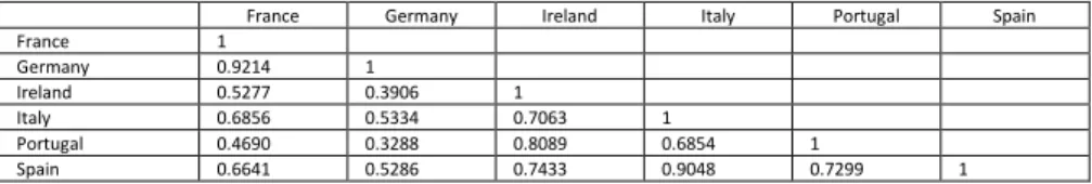
Table 2 reports Pearson’s correlation coefficients of the two-day rolling-average logarithmic bond yield changes. The greatest linear co-movement¹¹ of bond yield changes in the observed period was achieved between the French-German and between the Italian-Spanish sovereign bonds, while between the German- Portuguese and German-Irish sovereign bond yields the smallest correlation is observed.

Table 2

Pearson’s correlation of sovereign bond yield changes between Eurozone countries

France Germany Ireland Italy Portugal Spain

France 1

Germany 0.9214 1

Ireland 0.5277 0.3906 1

Italy 0.6856 0.5334 0.7063 1

Portugal 0.4690 0.3288 0.8089 0.6854 1

Spain 0.6641 0.5286 0.7433 0.9048 0.7299 1

Notes: all the correlation coefficients are significantly different from zero.

Following [1] an extreme positive yield change or exceedance is defined as the one that lies above the 95^th quintile of the marginal yield change distribution. In Table 3, the count numbers of exceedances and joint occurrences of extreme returns (co-exceedances) are reported. The results in Table 3 are presented as a lower triangular matrix, with the diagonal entries representing the number of exceedances in the particular country (because only the upper 5% of the extreme bond yield changes are of interest to the present study, there are

‖ ‖ exceedances). The other fields in the lower triangular matrix, presented in Table 3, are the counts of pair-wise co-exceedances of daily bond yield changes.

Table 3

Statistics of the counts of the (co-)exceedances of daily bond yield changes

France Germany Ireland Italy Portugal Spain

France 149

Germany 118 149

Ireland 71 68 149

Italy 97 80 77 149

Portugal 64 61 97 75 149

Spain 96 86 89 111 83 149

Notes: A total of 2,974 daily observations of two-day rolling window bond yield changes are observed. The numbers in the table can be explained as follows. For France, there were 149 occurrences (days) when the two-day rolling-window yield changes exceeded the 95^th quintile of the marginal yield change distribution in the total observed period. Further, there

10 The stationarity of bond yield changes was also examined, but the results (they lead to rejection of the unit root) are not relevant for this study, as I am interested only in the upper 5% of the bond yield changes distribution, and are thus not reported.

11 The Pearson’s correlation is a linear measure of comovement.

were 118 days of joint exceedances (i.e., co-exceedances) in the sovereign bond markets of France-Germany, 71 days of co-exceedances in France-Ireland sovereign bond markets, etc.

The greatest count of co-exceedances is achieved for the following pairs of national sovereign bond markets: Germany-France, Italy-Spain, France-Italy, and Ireland-Portugal. The lowest counts of sovereign bond markets are achieved for the pairs of France-Portugal and Germany-Portugal. Figure 1 in the Appendix illustrates the time series of (co-)exceedances for these pair-wise observed sovereign bond markets.¹²

Notably, in the period from mid-2000 to mid-2001 and in the year 2007, there were almost no exceedances or co-exceedances for the countries investigated and illustrated in Figure 1. After the global financial crisis began, in the third quarter of 2008, the count of (co-)exceedances across all observed pairs of sovereign bond markets increased. It is also evident that after the start of year 2010, the count of outcome 2 (exceedance) increased for the sovereign bond markets of France–

Portugal and Germany–Portugal and dominated over outcome 3 (co-exceedance).

This clearly indicates that extreme (positive) yield dynamics was achieved in only one of the countries in the investigated pair, namely Portugal. Judging just from Figure 1 and not controlling for the effects of the control variables, contagion in the sovereign bond markets would be identified when the counts of outcome 3 increased compared to non-crisis periods. Between the sovereign bond markets of France and Germany, contagion would then be identified in years 2003, 2009, and 2011 and between the sovereign bond markets of France and Italy in 2003 and 2009. Similarly, episodes of contagion in other sovereign bond markets could also be identified.

As argued in the Introduction and Section 2 of the present paper, to separate contagion from interdependence, one must control for the effects of the control variables. In the present paper, this is achieved by estimating multinomial logistic model (1). Results of the model are reported in Tables 4a and 4b.

Table 4a

Estimates of the multinomial logit regression model (1) for specific pair-wise observed sovereign bond markets

Fra-Ger Fra-Ire Fra-Ita Fra-Por Fra-Spa Ger-Ire Ger-Ita Ger-Por Outcome 2

Constant -4.881^a -3.4170^a -5.430^a -3.419^a -4.339^a 4.420^a -4.792^a -3.872^a

EUROSTOXX50 (returns)

53.650^a 13.341 7.945 16.080^c 19.766^c 25.304^a 16.066^c 25.499^a

cond. volatility of EUROSTOXX50 returns

148.895 359.471 325.581 262.860 619.915 175.443 186.174 238.669

EURIBOR (level) -0.029 -0.233^c 0.182 -0.219^c -0.224 -0.067 0.114 -0.188

12 In total I investigate (co-)exceedances for 15 ( ) pairs of national sovereign bond markets.

U. S. 10y T.N.

yield changes

90.870^a 56.763^a 59.529^a 60.727^a 51.617^a 53.234^a 74.889^a 62.105^a EUR-USD returns -23.302 -82.663^a -29.827 -96.70^a -118.543^a -41.258^b -19.897 -60.050^a

Crisis period 1 0.457 0.666^c 2.024^a 0.943^a 0.937^b 1.913^a 1.6234^a 1.625^a

Crisis period 2 1.707^a 2.373^a 3.402^a 2.366^a 2.911^a 3.474^a 3.050^a 2.984^a

Outcome 3

Constant -4.322^a -4.608^a -4.015^a -4.646^a -3.981^a -4.503^a -4.333^a -4.732^a

EUROSTOXX50 (returns)

45.774^a 21.124^b 20.135^b 26.707*^b 26.419^a 20.514^b 25.878^a 28.807^a cond. volatility of

EUROSTOXX50 returns

137.755 850.377^b 898.133^b 754.001^c 597.595 788.804^c 909.479^b 612.837

EURIBOR (level) -0.065 -0.040 -0.1148 -0.0703 -0.106 -0.0914 -0.1054 -0.0578 U. S. 10y T.N.

yield changes

131.133^a 108.138^a 120.650^a 106.758^a 113.659^a 115.404^a 122.586^a 108.948^a EUR-USD returns 3.979 -52.205^b -69.067^a 46.594^c -36.297 -47.287* -53.392^b -43.705

Crisis period 1 -0.064 -.0419 -1.146^a -0.069 -0.579 -0.630 -0.749^c 0.028

Crisis period 2 0.726^c 0.358 -0.913^c 0.195 -0.730 0.023 -0.772 0.247

Log likelihood -562.86 -715.22 -643.57 -718.59 -635.19 -669.04 -667.29 -681.90

LR chi (14) 464.67 455.87 462.49 476.30 485.63 560.34 510.97 560.14

Prob.>chi2 0.000 0.000 0.000 0.000 0.000 0.000 0.000 0.000

Pseudo-R² (McFadden)

0.292 0.241 0.264 0.249 0.277 0.292 0.277 0.291

Notes: Estimates of the regression coefficients of model (1) are given. EUROSTOXX50 (returns) are the two-day, rolling-average log returns of the EUROSTOXX50, whereas cond. volatility of EUROSTOXX50 returns are the EGARCH (1,1) conditional volatilities of the EUROSTOXX50 two-day rolling average log returns. U.S. 10y T. N. yield (log) changes are the two-day, rolling-average log changes of the U.S. Treasury note yields.

Crisis 1 is a time dummy for the first crisis period (September 16, 2008 – April, 22, 2010) and Crisis 2 is a time dummy of the second crisis period (from April 23, 2010 – August 31, 2011). Outcome 1 (no (co-)exceedance) is the base category. Outcome 2 presents the results of model (1) for category 2 (i.e., exceedance in one country only), whereas outcome 3 presents the results of model (1) for category 3 (i.e. co-exceedance). ^a/^b/^c denote the 1%, 5%, and 10% significance of the rejection of the null hypothesis that the regression coefficient is equal to 0, based on z-statistics. LR chi (14) reports the likelihood-ratio chi- square test (at 14 degrees of freedom) that for both equations (i.e., for outcome 2 and outcome 3) at least one of the covariate’s coefficients is not equal to zero. Prob. > chi2 reports the probability of getting a LR test statistic as extreme as, or more so, than the observed under the null hypothesis (i.e., that all of the regression coefficients across both models [i.e. for outcome 2 and outcome 3] are simultaneously equal to zero).

Table 4b

Estimates of the multinomial logit regression model (1) for specific pair-wise observed sovereign bond markets

Ger-Spa Ire-Ita Ire-Por Ire-Spa Ita-Por Ita-Spa Por-Spa

Outcome 2

Constant -4.777^a -4.054^a -4.109^a -4.098^a -3.148^a -5.316^a -3.682^a

EUROSTOXX50 (returns)

27.158^a 2.123 18.287^c 5.724 2.487 -0.794 5.080

cond. volatility of EUROSTOXX50 returns

297.095 455.702 281.783 82.863 277.361 150.641 260.602

EURIBOR (level) -0.064 0.004 -0.174 -0.104 -0.254^b 0.163 -0.196

USA 10y T.N.

yield changes

53.659^a 34.557^a 25.668^a 26.014^a 42.949^a 44.200^a 34.415^a

EUR-USD returns -78.945^a -54.392^a -72.904^a -80.411^a -87.045^a -23.325^a -112.409^a

Crisis period 1 1.765^a 1.085^a 1.719^a 1.466^a 0.649^c 2.014^a 1.117^a

Crisis period 2 3.495^a 2.695^a 2.537^a 2.826^a 1.962^a 2.885^a 2.434^a

Outcome 3

Constant -4.100^a -4.207^a -4.138^a -4.003^a -4.613^a -3.659^a -4.098^a

EUROSTOXX50 (returns)

31.068^a 4.055 3.402 8.336 11.189 8.601 15.328

cond. volatility of EUROSTOXX50 returns

534.693 1089.408^a 685.118^c 943.504^b 998.320^a 1026.443^a 789.804^b

EURIBOR (level) -0.138 -0.140 -0.127 -0.148 -0.026 -0.159 -0.154

USA 10y T.N.

yield changes

120.311^a 84.020^a 55.205^a 73.672^a 74.32333^a 75.43978^a 68.440^a EUR-USD returns -20.364 -132.768^a -116.402^a -112.486^a -117.266^a -126.023^a -102.325^a

Crisis period 1 0.536 -0.543 0.409 -0.319 0.255 -0.653^a 0.314

Crisis period 2 -0.770 0.827^c 2.172^a 1.311 1.345^a 0.821^b 1.433^a

Log likelihood -635.01 -754.90 -708.00 -722.17 -764.40 -677.96 -736.98

LR chi (14) 544.61 350.08 333.64 353.66 340.20 293.40 356.52

Prob.>chi2 0.000 0.000 0.000 0.000 0.000 0.000 0.000

Pseudo-R² (McFadden)

0.300 0.188 0.191 0.197 0.182 0.178 0.195

Notes: See notes for Table 4a.

I find that the regression coefficients of the EUROSTOXX50 returns, U.S. 10- year Treasury note yield changes, and for some pairs of sovereign bond markets, the EUR-USD returns and time dummies are significantly different from zero.

From the data in Table 4a, it follows that for the sovereign bond markets of France and Germany, a one unit (i.e., a 1%) increase in the EUROSTOXX50 returns is associated with a 0.536¹³ increase in the relative log odds of outcome 2 (i.e., exceedance in one of the sovereign bond markets) versus outcome 1 (i.e., no exceedance in any of the two observed markets). One can also see a 0.578 increase in the relative log odds of outcome 3 (i.e., co-exceedance) versus outcome 1. Similarly, a one unit increase (i.e., 1%) in U.S. 10-year Treasury note yields is associated with a 1.489 (1.311) increase in the relative log odds of outcome 2 (outcome 3). The pseudo- is between 0.18 and 0.30. For economic interpretation of the regression coefficients, however, one must calculate the marginal effects of the estimated coefficients ([12]). The marginal effects and probabilities of outcomes are reported in Tables 5a and 5b.

Turning first to estimated probabilities of outcomes, I find that the probabilities of joint extreme yield increases in the pair-wise investigated sovereign bond markets range between 0.0205 (or around 2%), for the sovereign bond markets of Germany–Portugal, and 0.0397 (or around 4%), for the sovereign bond markets of France-Germany, when not controlling for the covariates (see reported Probabilities 1 in Tables 5a and 5b).¹⁴ As noted, to separate contagion from interdependence, it is important to control for common and regional factors that impact all countries simultaneously. Evidently, this reduces the probabilities of observing outcome 3 (i.e., contagion) because it now ranges between 0.0083 for the sovereign bond markets of Germany–Portugal and 0.0168 for the sovereign bond markets of Ireland–Portugal (see Probabilities 2, reported in Tables 5a and

13 0.01*53.650, as in the data a 1% is expressed as 0.01.

14 If the outcomes were independent, then the probabilities of co-exceedances between all sovereign bond markets investigated pair-wise would be .

5b). The probability of observing no extreme yield moves in any of the two observed sovereign bond markets is the highest for France–Germany (0.9798) and lowest for Italy–Portugal (0.958). The probability of extreme yield movement in just one of the observed markets in the pair is the lowest for the bond markets of France–Germany (0.0088) and the highest for the markets of Ireland–Italy (0.0293). The results indicate that the sovereign bond yield dynamics of France and Germany were not only the most correlated (see Table 2) of all the markets investigated, but also had a very similar time path of extreme yield dynamics during the entire observed period.

Looking at specific covariates, EUROSTOXX50 returns, U.S. Treasury note yields, and EUR-USD exchange rate significantly impact the probability of extreme yield increases in the Eurozone sovereign bond markets. While positive EUROSTOXX50 returns and increased yields of U.S. Treasury notes increase the probability of extreme sovereign bond yield across the Eurozone, the increase in the EUR-USD exchange rate (i.e., appreciation of the EUR against the USD) significantly reduces the probability. The conditional volatility in the Eurozone stock markets and the money market interest rate do not significantly impact the probability of extreme yield movements in the Eurozone’s sovereign bond markets.

The responsiveness of the dependent (i.e., co-exceedance) variable to shocks in the Eurozone stock markets is not uniform across the sovereign bond markets. For example, a 1% increase in EUROSTOXX50 returns significantly (at the 5% level) increases the probability of extreme increase in bond yields in either the sovereign bond markets of France or Germany of 0.0046 (or 0.46%) and a probability of observing a contagion (i.e., a simultaneous extreme yield increase in both markets) of 0.0051 (or 0.51%). A similar response to shocks in the Eurozone stock markets are observed for the bond markets of Germany–Portugal and Germany–

Spain. In other pair-wise investigated sovereign bond markets, only the probability of outcome 2 or outcome 3 significantly increased; otherwise, the impact is insignificant (the latter can be noticed for the sovereign bond markets of Ireland–Italy, Ireland–Portugal, and Ireland–Spain). The increased volatility in the Eurozone stock markets significantly increases the probability of simultaneous extreme yield dynamics in the sovereign bond markets of France–Italy, Ireland–

Spain, Italy–Portugal, Italy–Spain, and Portugal–Spain.

Table 5a

Marginal effects and probabilities of outcomes for particular pair-wise observed sovereign bond markets

Fra-Ger Fra-Ire Fra-Ita Fra-Por Fra-Spa Ger-Ire Ger-Ita Ger-Por Outcome 2

EUROSTOXX50 (returns)

0.4648^a 0.3220 0.1115 0.4066^c 0.2337^c 0.4723^a 0.3106^c 0.5340^a cond. volatility

of EUROSTOXX50 returns

1.2866 8.6072 4.5548 6.5728 7.3644 3.1658 3.4873 4.9371

EURIBOR (level) -0.0002 -0.0057^b 0.00264 -0.0056^c -0.0027 -0.0012 0.0023 -0.0040 USA 10y T.N.

yield changes

0.7805^a 1.3656^a 0.8401^a 1.5341^a 0.6034^a 0.9815^a 1.4475^a 1.2937^a EUR-USD

returns

-0.2039 -2.0148^b -0.4195 -2.4714^a -1.4202^a -0.7678^b -0.3808 -1.2619^a Crisis period 1 0.0048 0.0210 0.0681^a 0.0344^b 0.0163 0.0780^a 0.0609^a 0.0650^a Crisis period 2 0.0309^c 0.1535^a 0.2218^a 0.1588^a 0.1306^a 0.2823^a 0.2184^a 0.2194^a Outcome 3

EUROSTOXX50 (returns)

0.5113^a 0.2028^b 0.2267^b 0.2287^b 0.3247^a 0.1744^c 0.2325^b 0.2312^b cond. volatility

of EUROSTOXX50 returns

1.5400 8.2095^c 10.1188^b 6.5010 7.3173 6.8400^c 8.2398^b 4.9732

EURIBOR (level) -0.0007 -0.0003 -0.0013 -0.0006 -0.0013 -0.0008 -0.0010 -0.0004 USA 10y T.N.

yield changes

1.4710^a 1.0412^a 1.357^a 0.9150^a 1.4018^a 0.9961^a 1.1015^a 0.8806^a EUR-USD

returns

0.0473 -0.4890^c -0.7773^a -0.3831 -0.4321 -0.4049^c -0.4821^b -0.3470 Crisis period 1 -0.0008 -0.0037 -0.0094^a -0.0009 -0.0061^c -0.0049^b -0.0056^b -0.0003 Crisis period 2 0.0103 0.0019 -0.0088^a 0.0001 -0.0080^b -0.0024 -0.0065^b -0.0001 Probabilities 1

Outcome 1 0.9395 0.9237 0.9324 0.9213 0.9321 0.9227 0.9267 0.9203

Outcome 2 0.0208 0.0525 0.0350 0.0572 0.0356 0.0545 0.0464 0.0592

Outcome 3 0.0397 0.0239 0.0326 0.0215 0.0323 0.0229 0.0269 0.0205

Probabilities 2

Outcome 1 0.9798 0.9650 0.9739 0.9649 0.9753 0.9720 0.9708 0.9701

Outcome 2 0.0088 0.0252 0.0147 0.0264 0.0122 0.0192 0.0200 0.0216

Outcome 3 0.0114 0.0099 0.0115 0.0088 0.0126 0.0088 0.0092 0.0083

Notes: Probabilities 1 are probabilities of outcomes when one does not control for covariates. Probabilities 2 are probabilities of outcomes after controlling for the covariates and are calculated by Equation (4). ^a/^b/^c denote the 1%, 5%, 10% significance of the rejection of the null hypothesis that the marginal effect of the covariate is equal to 0 based on z-statistics. The reported marginal effects of the time dummy covariates (Crisis period 1, Crisis period 2) show by how much the probability of observing outcome 2 (outcome 3) increases when the value of the time dummy variable changes from 0 to 1.

A significant impact on the probability of extreme yield increases in all the Eurozone’s sovereign markets is exerted by the yield dynamics of the U.S.

Treasury notes. For instance, a 1% increase in the yields of U.S. Treasury notes increases the probability of an extreme increase in the yields in the sovereign bonds of either France or Germany by 0.78% and the probability of contagion between the bond markets of France and Germany by 1.47%.

Appreciation of the euro against the U.S. dollar reduces the probability of extreme increases in the yields of Eurozone sovereign bond markets, except in the markets of France–Germany. The negative relationship between the exchange rate and sovereign bond yields dynamics can be explained as follows. Increased EUR-USD exchange rate increases the demand for Eurozone bonds as the expected return on the euro denominated bond investment increases. Increased demand for bonds, in turn, increases their prices and reduces their yields. The marginal effect of covariate is significantly different from zero across all the pair-wise observed sovereign bond markets.

Table 5b

Marginal effects and probabilities of outcomes for particular pair-wise observed sovereign bond markets

Ger-Spa Ire-Ita Ire-Por Ire-Spa Ita-Por Ita-Spa Por-Spa

Outcome 2 EUROSTOXX50 (returns)

0.3621^a 0.0589 0.3113^c 0.1116 0.0657 -0.01339 0.1066

cond. volatility of EUROSTOXX50 returns

3.9344 12.5523 4.6130 1.3537 7.4200 1.8063 5.4658

EURIBOR (level) -0.0008 0.0002 -0.0029 -0.0020 -0.0071^b 0.0023 -0.0043

USA 10y T.N. yield changes

0.7073^a 0.9514^a 0.4223^a 0.4957^a 1.1792^a 0.5924^a .7338^a

EUR-USD returns -1.0622^a -1.4973^a -1.2112^a -1.5689^a -2.4025^a -0.2888 -2.4376^a

Crisis period 1 0.0493^b 0.0464^b 0.0581^a 0.0522^b 0.0229 0.0650^b 0.0373^b

Crisis period 2 0.2243^a 0.221^a 0.1181^a 0.1809^a 0.1172^a 0.1412^a 0.1425^a

Outcome 3 EUROSTOXX50 (returns)

0.3053^a 0.0482 0.0508 0.1262 0.1427 0.1658 0.2234

cond. volatility of EUROSTOXX50 returns

5.2769 12.9953 11.2122^c 14.4642^b 12.7120^b 19.714^a 11.511^b

EURIBOR (level) -0.0014 -0.00169 -0.0021 -0.0022 -0.0002 -0.0031 -0.00219

USA 10y T.N. yield changes

1.1891^a 1.0025^a 0.9026^a 1.1232^a .9380^a 1.4398^a 0.9935^a

EUR-USD returns -0.1917 -1.5842^a -1.8977^a -1.7020^a -1.4727^a -2.4191^a -1.4650^a

Crisis period 1 -0.0048^c -0.0059^c 0.0064 -0.0050 0.0032 -0.0109^b 0.0044

Crisis period 2 -0.0071^a 0.0083 0.0786^a 0.0259^c 0.0254^c 0.0162 0.0310^b

Probabilities 1

Outcome 1 0.9287 0.9257 0.9324 0.9297 0.9250 0.9371 0.9277

Outcome 2 0.0424 0.0484 0.0350 0.0403 0.0498 0.0256 0.0444

Outcome 3 0.0289 0.0259 0.0326 0.0299 0.0252 0.0373 0.0279

Probabilities 2

Outcome 1 0.9763 0.9585 0.9659 0.9640 0.9580 0.9663 0.9626

Outcome 2 0.0137 0.0293 0.0174 0.0204 0.0289 0.0141 0.0225

Outcome 3 0.0100 0.0122 0.0168 0.0156 0.0130 0.0196 0.0149

Notes: See notes for Table 5a.

To answer the question of whether the probability of contagion increased during the global financial crisis and the Eurozone debt crisis, the marginal effects of the dummy variables of Crisis period 1 and Crisis period 2 must be analyzed. The time-dummy covariates significantly impact the probability of (co-)exceedances across the pair-wise observed markets, except the sovereign bond markets of France–Germany. The probability of observing exceedance (i.e., outcome 2) during the Eurozone debt crisis increased dramatically compared to the pre-crisis period. For example, the probability of extreme upside movement in sovereign bond yields increased by 0.28 (or 28%) compared to the pre-crisis period when simultaneously analyzing Germany’s and Ireland’s exceedance time series. The probability of observing co-exceedance (i.e., outcome 3) of extreme positive bond yield changes during the Eurozone debt crisis increased for the sovereign bond markets of Ireland–Portugal and for Portugal–Spain, whereas the probability reduced for the markets in France–Spain and Germany–Spain. The estimates of the marginal effects of the time dummies indicate less synchronous extreme yield dynamics across the Eurozone sovereign bond markets during the global financial crisis and especially during the Eurozone debt crisis compared to the pre-crisis periods.

Responses of the probability estimates to the full range of values associated with different covariates are computed and graphically presented in Figures 2a (for the France–Germany) and 2b (for Germany–Portugal).

Notes: Marginal effects are calculated by Equation (5).

Figure 2a

Co-exceedance response curves of the sovereign bond markets of France-Germany to changes in covariates

The probability of (co-)exceedance in bond markets clearly increases with the stock market returns, but it does so nonlinearly. Stock market volatility increases the probability of (co-)exceedance only after it reaches some threshold. From Figures 2a and 2b, this is when conditional variance exceeds 0.0015 a day. The U.S. Treasury note yield increases highly increase the probability of co- exceedances in the Eurozone bond markets when yields in the U.S. bond market increase by more than 0.02 (2%) a day, whereas the EUR-USD returns increase the probability of co-exceedance between the bond markets of Germany-Portugal when the exchange rate falls by more than 1% a day.

0.2.4.6.8 1

Probability

-.05 0 .05

EUROSTOXX50 returns

Outcome 1 Outcome 2

Outcome 3

Co-exceedance response curve for the EUROSTOXX50

0.2.4.6.8 1

Probability

0 .001 .002 .003

EUROSTOXX conditional volatility

Outcome 1 Outcome 2

Outcome 3

Co-exceedance response curve for EUROSTOXX50 cond. volatility

0.2.4.6.8 1

Probability

-.1 -.05 0 .05 .1

U.S. Treasury notes daily yield changes

Outcome 1 Outcome 2

Outcome 3

Co-exceedance response curve for the U.S. Treasury notes

0.2.4.6.8 1

Probability

-.02 -.01 0 .01 .02 .03

EUR-USD returns

Outcome 1 Outcome 2

Outcome 3

Co-exceedance response curve for the EUR-USD returns

Notes: Marginal effects are calculated by Equation (5).

Figure 2b

Co-exceedance response curves of the German-Portugal’s sovereign bond markets to changes in covariates

Conclusion

In the present paper, a multinomial logistic model was applied to analyze contagion between six Eurozone countries based on a measure of joint occurrences of large yield changes (i.e., co-exceedances), controlling for developments in common and regional factors that affect all sovereign bond market simultaneously. I found that Eurozone stock markets (EUROSTOXX50 returns), U.S. Treasury note yields and the EUR-USD exchange rate significantly impact the probability of extreme yield moves in the Eurozone sovereign bond markets. Whereas positive EUROSTOXX50 returns and positive U.S. Treasury note yield moves increase the probability of extreme positive sovereign bond yields in the Eurozone sovereign bond markets, appreciation of the euro against the U.S. dollar significantly reduces the probability. The conditional volatility in the Eurozone stock markets and the money market interest rate do not

0.2.4.6.8 1

Probability

-.05 0 .05

EUROSTOXX50 returns

Outcome 1 Outcome 2

Outcome 3

Co-exceedance response curve for theEUROSTOXX50

0.2.4.6.8 1

Probability

0 .001 .002 .003

EUROSTOXX_cond_vol_EGARCH

Outcome 1 Outcome 2

Outcome 3

Co-exceedance response curve for the EUROSTOXX50 cond. volatility

0.2.4.6.8 1

Probability

-.1 -.05 0 .05 .1

log_US_tresury_notes_10y

Outcome 1 Outcome 2

Outcome 3

Co-exceedance response curve for U.S. Treasury notes yield changes

0.2.4.6.8 1

Probability

-.02 -.01 0 .01 .02 .03

log_EUR_USD Outcome 1 Outcome 2 Outcome 3

Co-exceedance response curve for the EUR-USD returns

significantly impact the probability of extreme yield movements in the Eurozone’s sovereign bond markets.

The probability of observing exceedance during the Eurozone debt crisis increased dramatically compared to the pre-crisis periods. The probability of observing co- exceedance of extreme positive bond yield changes during the Eurozone debt crisis increased for the sovereign bond markets of Ireland–Portugal and Portugal- Spain, whereas the probability reduced for the markets in France–Spain and Germany-Spain. The results indicate a less synchronous extreme yield dynamic across the Eurozone sovereign bond markets during the global financial crisis and especially during the Eurozone debt crisis compared to a pre-crisis period.

The results of the present study might be of interest for policymakers, central banks, and investors in financial markets. Through contagion analysis, one gains knowledge of whether a shock in one segment of a national financial market is transmitted across markets via channels that appear only during turbulent periods or whether these shocks are transmitted via channels or inter-linkages that exist in all states of the world (non-crisis as well as crisis periods).

References

[1] Bae, K. H, Karolyi, G. A. and Stulz, R. M. (2003) ‘A New Approach to Measuring Financial Contagion’, Review of Financial Studies, 16(3), pp.

717-763

[2] Baur, D. G. and Lucey, B. M., (2009) ‘Flights and Contagion - An Empirical Analysis of Stock-Bond Correlations, Journal of Financial Stability 5(4), pp. 339-352

[3] Baur, D. and Schulze, N. (2005) ‘Coexceedances in Financial Markets - A Quantile Regression Analysis of Contagion’, Emerging Markets Review, pp. 5(1), 21-43

[4] Corsetti, G., Pericoli, M. and Sbracia, M. (2001) ‘Correlation Analysis of Financial Contagion: What One Should Know Before Running a Test’.

Economic Growth Center, Yale University Discussion Paper No. 822 [5] Dornbusch, R., Park, Y. C. and Claessens, S. (2001) ‘Contagion: Why

crises spread and how this can be stopped’, in Claessens, S., and Forbes, K. (Eds.), International Financial Contagion, Kluwer Academic Publishers, Boston, pp. 19-42

[6] Dungey, M., Fry, R., Gonazlés-Hermosillo, B. and Martin, V. L. (2005)

‘Empirical Modelling of Contagion: A review of Methodologies’, Quantitative Finance 5(1), pp. 9-24

[7] Dungey, M., and Martin, V. L. (2007) ‘Unraveling Financial Market Linkages during Crises’, Journal of Applied Econometrics, 22(1), pp. 89- 119

[8] Durré, A. and Giot, P. (2005) ‘An International Analysis of Earnings, Stock Prices and Bond Yields’. European central bank working paper No. 515 [9] Forbes, K. J. and Rigobon, F. (2001) ‘Measuring contagion: Conceptual

and empirical issues’, in Claessens, S., and Forbes, K. (Eds.), International Financial Contagion, Kluwer Academic Publishers, Boston, 43-66

[10] Forbes, K. and Rigobon, R. (2002) ‘No Contagion, Only Interdependence:

Measuring Stock Market Co-movements’, Journal of Finance 57(5), pp.

2223-61

[11] Gravelle, T., Kichian M. and Morley, J. (2006) ‘Detecting Shift Contagion in Currency and Bond Markets’, Computing in Economics and Finance 2002, 58. Society for Computational Economics

[12] Greene, W. H. (2003) ‘Econometric Analysis’, 5^th ed., Prentice Hall, New Jersey

[13] Kim, S. and In, F. (2007) ‘On the Relationship in Stock Prices and Bond Yields in the G7 Countries: Wavelet analysis’, Journal of International Financial Markets, Institutions and Money, 17(2), pp. 167-179

[14] Longin, F. M. and Solnik, B., (1995) ‘Is the Correlation in International Equity Returns Constant: 1970-1990?’, Journal of International Money and Finance, 14(1), pp. 3-26

[15] McFadden, P. (1974) ‘The Measurement of Urban Travel Demand’, Journal of Public Economics, 3(4), pp. 3303-3328

[16] Metiu, N. (2011) ‘Financial Contagion in Developed Sovereign Bond Markets’. METEOR – Maastricht Research School of Economics of Technology and Organization, Research Memoranda 004

[17] Nelson, D. B. (1991) ‘Conditional Heteroskedasticity in Asset Returns: A New Approach’, Econometrica, 59(2), pp. 347-370

[18] Pericoli, M. and Sbracia, M. (2003) ‘A Primer on Financial Contagion’, Journal of Economic Surveys, 17(4), pp. 571-608