Solvency risk minimizing guaranteed returns in life insurance

(1)

Solvency risk minimizing

guaranteed returns in life insurance by Borbála Szüle

C O R VI N U S E C O N O M IC S W O R K IN G P A PE R S

CEWP 2 /201 6

(2)

Solvency risk minimizing guaranteed returns in life insurance

Borbála Szüle

^∗

January 11, 2016

Abstract

Return guarantee constitutes a key ingredient of classical life insurance premium calculation. In the current low interest rate environment insurers face increasingly strong financial incentives to reduce guaranteed returns embedded in life insurance contracts. However, return guarantee lowering efforts are restrained by associated demand effects, since a higher guaranteed return makes the net price of the insurance cover lower. This tradeoff between possibly higher future insurance obligations and the possibility of a larger demand for life insurance products can theoretically also be considered when determining optimal guaranteed returns. In this paper, optimality of return guarantee levels is analyzed from a solvency point of view. Availability and some other properties of optimal solutions for guaranteed returns are explored and compared in a simple model for two measures of solvency risk (company-level and contract-level VaR). The paper concludes that a solvency risk minimizing optimal guaranteed return may theoretically exist, although its practical availability can be impeded by economic and regulatory constraints.

Keywords: Risk Analysis, Insurance JEL: G11, G22

1 Introduction

Traditional life insurance premium calculation shares important features with financial valuation methods: an essential part of the calculation is the quantification of discounted (probability adjusted) cash flow values. Under the

∗Insurance Education and Research Group, Corvinus University of Budapest, Email:

borbala.szule@uni-corvinus.hu

(3)

equivalence premium principle, that traditionally constitutes the basis for net premium calculation in life insurance, the expected present value of paid benefits equals the expected present value of net premium income for a certain type of insurance contract e. g. Banyár(2003) page 185, Dickson et al.

(2011) page 146). The interest rate applied to calculate these present values (sometimes also referred to as technical rate of return) can be considered as a guaranteed return. To safeguard solvency of insurance companies, the maximum possible guaranteed returns are generally also fixed by regulation, in Hungary this maximum rate was 2,9 % in July 2015 (61/2013. (XII. 17.) NGM r.) which is lower than previously, for example as of 15th July 2000, when the maximum rate was 5,5 % (CEIOPS (2005)).¹

To some extent, guaranteed returns in life insurance are also related to the market rate of return. This relationship have already been incorporated into theoretical microeconomic models by assuming the application of an actuarially fair interest rate (e. g. Yaari (1965)), or for example with the application of market rate related interest in numerical calculations (Borch (1980). It is worth mentioning that, in practice, guaranteed returns for a life insurance policy are usually less than the market rate for risk-free assets of the same maturity (Briys-de Varenne (1997)), and thus the guaranteed return can be considered as a conservative estimate of future investment earnings (Holsboer (2000)).

The incorporation of guaranteed returns into traditional life insurance premium calculation can be financially risky for life insurance companies if market interest rates decrease persistently. Previous studies confirmed that the recent low interest rate environment has made it more challenging for life insurance companies to manage their assets and liabilities (e.g. Berend et al. (2013)), and that traditional life insurance return guarantees may have substantial market value (e.g. Persson-Aase (1997)). Empirical studies also point to a potential life insurance solvency risk in the prevailing period of low interest rates (e.g. Kablau-Weiß (2014),EIOPA (2014)).

Recently, the solvency of insurance companies is a central issue in the European Union, where the new Solvency II rules (regulation about insurance company solvency) are expected to be introduced in 2016. There are numerous measures for solvency risk, either related to the calculation of fail- ure probabilities (e.g. Barnhill-Schumacher (2011)), or associated with an other method, for example with the calculation of regulatory capital ratios (e.g. Pierret (2015)). Literature also mentions the concept of Value-at-Risk

1In some other European Union countries there have also been developments in determining the guaranteed interest rates applied in life insurance premium calculation: for example (with effect from 1st January 2011) Denmark lowered this rate for new life insurance contracts from 2 % to 1 %. (EIOPA(2011))

(4)

(VaR) as having become a standard risk measure used to evaluate exposure to risk in an institution. (Panjer(2001)) VaR can be interpreted as the amount of capital required to ensure that a specific institution (for example insurance company or bank) does not become technically insolvent (with an adequately high degree of certainty). (McNeil (2005) pages 43-44, Panjer (2001)) CEA – Mercer Oliver Wyman (2005) show that the majority of surveyed insurance solvency assessment models applied the standard VaR approach, with the Swiss Solvency Test applying Tail VaR², being the only exception among the surveyed models. VaR is also a key risk measure in the new Solvency II regulation in the quantification of solvency capital requirements. (Directive 2009/138/EC, Article 101)

In this paper company-level (total) VaR and contract-level VaR are calculated to measure solvency capital requirement, which can be considered as a measure of solvency risk.³ The key research question of the paper is, whether theoretically a solvency risk minimizing guaranteed return can be found, if potential demand effects of guaranteed return choices are also taken into account. A potential reason for a demand effect may be that (according to the mathematics of equivalence principle based premium calculation method), the net price of the life insurance cover (the net premium) is lower, if the guaranteed return is higher. Thus, fierce competition in the insurance industry may result in high guaranteed returns. (BIS (2011)) Empirical research results also revealed that prince sensitivity of consumer demand for certain types of life insurance may be non-negligible (e.g. Babbel (1985)).⁴ Demand for life insurance may be measured with the number of insurance policies sold by insurance companies. Since with a larger set of insurance contracts (with the same main properties) the variance of profit may be lower, the demand for an insurance product (measured as the number of sold insurance policies) may also have an impact on the solvency of an insurance companies.

There are thus (at least in a simple theoretical model) two channels how guaranteed returns in life insurance may affect solvency risk. After recog- nizing these relationships, the question also arises whether theoretically an optimal (solvency risk minimizing) guaranteed return exists. The paper ex-

2For continuous loss distribution functions TailVaR and Expected Shortfall refer to the same value, and Expected Shortfall can be interpreted as the expected value of loss if the loss is higher than VaR. (McNeil et al. (2005), pages 44-45.)

3Solvency risk could also be called „insolvency risk”, since both expressions can be considered as referring to the same phenomenon (that the insurance company becomes insolvent, which means that the insurance company can not remain solvent).

4Although it has to be emphasized that the existence of strong price elasticity of demand for life insurance is not automatically equivalent to a high degree of price competition in life insurance industry. (Babbel(1985))

(5)

tends the literature on life insurance guaranteed returns by analyzing this research questions in a simple model that also highlights possible demand effects of guaranteed return choices. According to the results of the paper, the existence of such an optimal guaranteed return is possible, although the practical availability of the optimum can be restricted as a consequence of economic and regulatory constraints.

The paper is organised as follows. Section 2 introduces the theoretical model of the insurance company constructed to analyze the research question.

Section 3 provides a description of the solvency risk measures in the paper, and Section 4 presents theoretical results about optimal guaranteed returns.

Section 5 concludes and describes directions for future research.

2 The model

The model aims at involving the most important features of insurance companies selling classical life insurance products.⁵ Among life insurance contract types, a traditional distinction can be made between the conctracts whereby the insurance company guarantees a specific return to the policyholder, and the unit-linked contracts (without guaranteed return). (BIS (2011)) In the paper only classical life insurance products with guaranteed returns are modeled. The distinction between these types of contracts is relevant also from the point of view of solvency: according to the new Solvency II rules capital requirements may be lower for unit-linked insurance products, as in case of many unit-linked products investment risk is borne by policyholders. (ECB (2007), page 7)

According toInsurance Europe(2014) (page 23) the majority of assets on the asset side of balance sheets of insurance companies is related to bonds, and the largest component on the other side of the balance sheet is associated with insurance liabilities. This balance sheet structure can be considered as a consequence of "classical" insurance features: traditionally insurance companies take insurance risks, receive premium payments and invest the majority of collected premiums (mainly into bonds). A stylized balance sheet for an insurance company is presented on Figure 1.

The insurance portfolio consists of individual contracts that are assumed to be similar in the model: it is assumed that the probability belonging to the occurrence of the insurance event (p) is the same for each insurance policy.

For each individual insurance policy the following random variable can be defined:

5To some extent, non-life insurance differs from life insurance.

(6)

Invested assets

Equity Insurance

liabilities

Figure 1: Stylized balance sheet

ξ_i =

(1 if the insurance event occurs

0 otherwise (1)

On company level, the sum of the random variables defined in Equation (1) equals the total number of occured insurance event:

ξ =ξ₁+. . .+ξ_n (2)

The random variable in Equation (2) is binomially distributed, and its distribution function can be approximated with the normal distribution function for a sufficiently large insurance portfolio.⁶

In practice, an insurance contract can be quite complex, this model however concentrates on the most important features of insurance contracts: it is assumed that on the one hand the policyholder pays a single premium (net premium plus certain expenses) and on the other hand policyholders are en- titled to receive the sum insured (B) if the insurance event occurs during the term of the insurance. It is assumed that the insurance is issued with a one year term. The guaranteed return (technical rate of return) belonging to the insurance contracts is indicated by i in the model. Based on these assumptions, and with the application of the equivalence principle⁷, the net premium payable by the policyholder at the beginning of the insurance term equals

Bp

1+i. At the beginning of the insurance term the sum of collected net premiums equals the value of insurance reserves (that correspond to insurance

6It can be assumed in the model that the number of insurance contracts is higher than the number that is required to a good approximation with the normal distribution function.

7The equivalence principle is described by for example Banyár (2003) (on page 185) andDickson et al. (2011) (on page 146).

(7)

liabilities). The number of insurance contracts depends on the guaranteed return and is indicated byn(i)in the model. It is also assumed that (according to usual microeconomic assumptions) if the insurance premium is lower (as a consequence of a higher guaranteed return), then the demand for the specific insurance type is higher, that can be formulated as ^∂n(i)_∂i > 0. The paper does not aim to explore possible price competition issues within the insurance industry, the presented analysis focuses on a single insurance company for which the size of the insurance portfolio (the number of insurance contracts) depends on the value of guaranteed return.

Beside insurance liabilities, the insurance company is assumed to have own funds (equity) as well, and without loss of generality it can be assumed that equity is defined as ^sBp_1+i with the application of a „solvency multiplier”

indicated by s.⁸

In the model, it is also assumed that at the beginning of the insurance term the collected net premiums and the equity are invested into financial assets that correspond to regulatory requirements for insurance company investment. As indicated by Insurance Europe (2014) (page 23) a large part of assets on the asset side of balance sheets of insurance companies is related to bonds. The expected value of the return on these investments can be assumed to be higher than the guaranteed return. In practice, excess return sharing (over the guaranteed return) is often also regulated (the insurance company receives only a part of the excess return). That part of the return on the financial investments, that belongs to the insurance company (with taking into account return sharing rules as well), is indicated by r in the model. Since the presented analysis concentrates on the choice of guaranteed returns,ris not assumed to be a random variable (although it can be assumed thatr is higher thani). The discounting rate is indicated byk. According to Panjer (2001) the distribution of the present value of losses can be modeled when solvency measures are calculated for lines of business of an insurance company. The present value of loss in this model is described by Equation (3):

η= Bξ

1 +k −n(i) Bp 1 +i

(1 +s)(1 +r)

1 +k (3)

8In a simple form, this expression corresponds to solvency requirements that are influ- enced by the total risk exposure of an insurance company.

(8)

3 Solvency risk measures

Theoretically, there are several measures of solvency risk, and the definition of a solvency risk measure may also depend on the context where risk is measured. When analyzing banking sector data, Pierret (2005) for example mentions regulatory capital ratios, certain market measures of risk (market beta and realized volatility), and a measure of the expected capital shortfall as solvency risk measures. In an insurance sector related analysis VaR can also be considered as an adequate measure that quantifies solvency risk.

The growing importance of VaR in the insurance sector is related to the new Solvency II regulation, where VaR is applied as a measure for solvency capital requirements, with declaring that (Directive 2009/138/EC, Article 101):

"It shall correspond to the Value-at-Risk of the basic own funds of an insurance or reinsurance undertaking subject to a confidence level of 99,5% over a one-year period."

In the following company-level and contract-level VaR are considered as alternative solvency measures in the paper.

VaR is an amount that may be interpreted as a random variable feature.

As a consequence of the random nature of insurance events the insurance company is exposed to insurance risk: the number of contracts, whereon the insurance company has to pay the sum insured, is a random variable.

Since the present value of loss in Equation (3) is a (linear) function of the sum of insurance events in the model, it is also a random variable with normal distribution. According to McNeil et al. (2005) (page 39) the mean and standard deviation of a normally distributed variable, together with the confidence level, is sufficient to calculate VaR. The mean present value of loss is n(i)_1+k^Bp(1− ^(1+s)(1+r)_1+i ) and the variance is _1+k^Bp2

n(i)p(1−p). The Value-at-Risk (VaR) belonging to the present value of loss (at α confidence level) is calculated by Equation (4). In line with McNeil et al. (2005) (page 39), to emphasize the effect of guaranteed return on the result, in Equation (4) it is also indicated that company level VaR depends on the value of the guaranteed return in the model:

V aR(i) =n(i) Bp 1 +k

1− (1 +s)(1 +r) 1 +i

+ + Φ⁻¹(α) B

1 +k

pn(i)p(1−p)

(4)

(9)

To ensure simplicity and unambigousity of notations, in the following expressions and graphs VaR indicates a company-level value, while it is clearly signified when a result is related to contract-level VaR.

The influence of guaranteed return on life insurance demand is a key assumption in the model, as explained more in detail in the previous section.

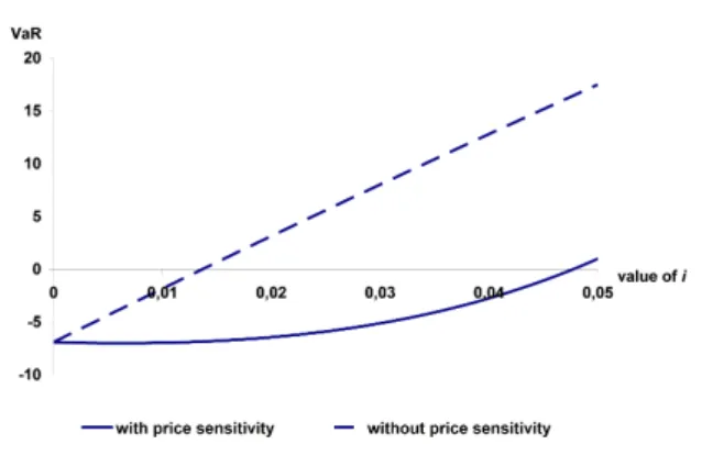
The importance of this assumption is illustrated by Figure 2, where a numerical example demonstates the potentially large difference in VaR functions with and without the assumption of a guaranteed return dependent life insurance demand. In the following, in the numerical examples it is assumed that the number of insurance contracts (that can be considered as a measure of life insurance demand) is described by Equation (5), where g > 0 and c > 0:

n(i) = c(1 +i)^g. (5)

This assumption about the size of the insurance portfolio can be interpreted in a way that life insurance demand is not only explained by the guaranteed return, but if the guaranteed return is higher, a larger demand for life insurance may be observed. It also means that without assuming price sensitivity of life insurance demand, the number of insurance contract is a constant value (that does not depend on the value of guaranteed return). Figure 2 illustrates how significantly VaR may change if price sensitivity assumption is introduced in the model (B = 1, i = 0.01, p = 0.05, s = 0.1, k = 0.1, α = 0.995, r= 0.025, c= 10000,g = ⁵⁰₃).

Figure 2: Effect of price sensitivity on solvency risk Source: own calculations

A possible alternative solvency measure in the model is contract-level VaR

(10)

that can be defined as q(i) = ^{V aR(i)}_n(i) . Equation (6) presents the definition of contract-level VaR in the model:

q(i) = Bp 1 +k

1− (1 +s)(1 +r) 1 +i

+ + Φ⁻¹(α) Bp

1 +k

pp(1−p) 1 pn(i)

(6)

Figure 2 shows that the sign of company-level VaR, and thus also that of contract-level VaR, may be positive or negative as well. With recalling that the loss variable has a normal distribution, a negative VaR in case of the loss present value (that belongs to a relatively high confidence level) can be interpreted so that the theoretical mean of loss is also negative, that also indicates that the theoretical mean of the profit is a positive value (and it can be considered as advantageous for an insurance company from an economic point of view). If the VaR of loss is higher, it can be considered as less advantageous for the insurance company in the model, since in this case solvency risk is higher. In this model framework VaR is only interpreted as a measure of solvency risk. Although (in an adequately designed model framework) VaR values could also be interpreted as solvency capital requirement, it has to be emphasized, that in this model the insurance company is assumed to have an amount of capital that is enough to fulfil regulatory requirements (it means that the value of the „solvency multiplier”, indicated by s in the model, is assumed to be sufficiently high).

4 Optimal guaranteed returns

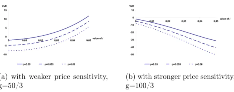
Changes in the value of guaranteed return can theoretically increase or decrease company-level or contract-level VaR. These effects on company-level VaR are illustrated by Figure 3 for different insurance event occurrence probabilities (B = 1,i= 0.01,s= 0.1,k= 0.1,α = 0.995,r = 0.015,c= 10000).

Figure 3 indicates that the extent of price sensitivity of demand has an important effect on how guaranteed returns influence company level VaR:

if in Equation (5) g = ⁵⁰₃, then a higher guaranteed return results in a higher company-level VaR, while for g = ¹⁰⁰₃ in Equation (5) the opposite relationship may be observed in the numerical example.

In spite of the relatively simply model framework, the effect of guaranteed return on VaR may be quite complex. The first order derivate of the company-level VaR function in Equation (4) is presented by Equation (7).

(11)

(a) with weaker price sensitivity, g=50/3

(b) with stronger price sensitivity, g=100/3

Figure 3: Effect of event probability on solvency risk Source: own calculations

∂V aR(i)

∂i = Bp

1 +k

∂n(i)

∂i

1− (1 +s)(1 +r) 1 +i

+ + Bp

1 +k

∂n(i)

∂i Φ⁻¹(α)p

n(i)p(1−p)1 2

1 pn(i)

! + +n(i)(1 +s)(1 +r)

(1 +i)²

(7)

If it is assumed that both ^∂n(i)_∂i > 0 and ^∂²_∂iⁿ⁽ⁱ⁾2 > 0 then it is possible that a minimum in the company-level VaR function exists (since then it is possible that for a certain guaranteed return value ^{∂V aR(i)}_∂i = 0 and ^∂²^{V aR(i)}_∂i2 >0. The optimal guaranteed return value that minimizes company-level VaR (if such an optimization is possible) can be calculated from solving Equation (8):

n(i) (1 +i)²

(1 +s)(1 +r)(1 +k)

Bp = ∂n(i)

∂i

(1 +s)(1 +r) 1 +i

− ∂n(i)

∂i

Φ⁻¹(α)p

n(i)p(1−p) 2p

n(i)

!

− ∂n(i)

∂i

(8)

Although a solvency risk minimizing guaranteed return may exist, it also has to be emphasized that the existence of a company-level VaR minimizing guaranteed return depends also on the parameter values, and it is also possible that such a minimum does not exist. An optimal result for a numerical example (B = 1, i = 0.01, s = 0.1, k = 0.1, p= 0.0275, α = 0.995, r = 0.0125, c= 10000, g = ¹¹⁰₃ ) is illustrated on Figure 4:

(12)

Figure 4: Eﬀect of guaranteed return on VaR Source: own calculations

Equation (8) may have more than one solutions, and it is also possible that for one of the solutions the company-level VaR function has a (local) maximum and for an other solution the company-level VaR is minimal. For an economically correctly interpretable solution the optimal (VaR minimizing) guaranteed return should not be a negative number. In addition to this, an other constraint should also be taken into consideration: in practice a legally defined maximum value for guaranteed returns exist. By summa- rizing the criteria for an optimal solution, one can conclude that a VaR minimizing guaranteed return may be considered as „available”, if it is within a relatively narrow interval, where the interval is defined by economic and regulatory constraints. Figure 4 also illustrates that even if a company-level VaR minimizing optimal guaranteed return exists, it may not be available if the possible maximum guaranteed return defined by regulation is lower than the mathematically optimum value.

Beside company-level VaR, contract-level VaR is also a possible solvency risk measure. The ﬁrst derivative of q(i) = ^{V aR}_n₍_i⁽₎ⁱ⁾ describes how changes in guaranteed return aﬀect contract-level VaR:

∂q(i)

∂i = Bp(1 +s)(1 +r)

(1 +i)²(1 +k) − ∂n(i)

∂i

Φ⁻¹(α)B

p(1−p) 2(1 +k)

n(i)³ (9) By setting the expression in Equation (9) equal to zero the condition that deﬁnes optimal (contract-level VaR minimizing) guaranteed returns can be calculated, as described by Equation (10).

(13)

(a) p=0.0275 (b) p=0.0235

(c) p=0.035

Figure 5: Different optimum levels Source: own calculations

(1 +i)² pn(i)³

∂n(i)

∂i = 2 r p

1−p

(1 +s)(1 +r)

Φ⁻¹(α) (10)

Similar to company-level VaR, it is also possible that Equation (10) does not have an „available” solution. The second order derivative ofq(i) = ^{V aR(i)}_n(i) may be positive while Equation (10) holds, but it is also possible that a contract-level VaR minimizing guaranteed return does not exist, or even if it exists, it is not within the interval defined by economic and regulatory constraints.

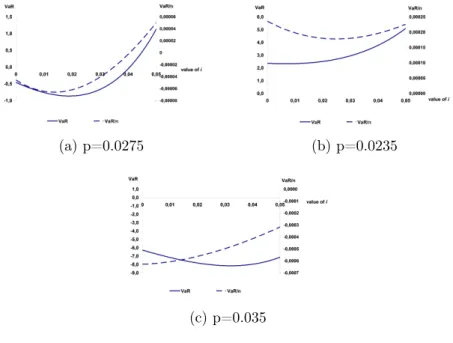
If a contract-level VaR minimizing optimal guaranteed return exists, it may be higher or lower than the company-level VaR minimizing optimum value. In a numerical example (for different insurance event probabilities) Figure 5 shows three cases in which these optimum values differ (B = 1, i= 0.01, s= 0.1, k = 0.1,α = 0.995, r= 0.05, c= 10000, g = ⁵⁰₃ ).

Figure 5 also illustrates that even if a solvency risk minimizing optimal guaranteed return exists mathematically, it may be inavailable practically, if the optimum value is higher than the regulatory maximum value.

For a number of reasons, it could be problematic to develop practical business decisions based on these mathematical resuls. First of all, it is

(14)

mathematically possible that there is no solvency risk minimizing optimum that is not a negative value. Furthermore, the optimal solution should ideally be lower than the legally defined maximum guaranteed return. In addition to this, the choice of risk measures can also influence the results. Together with these limitations, one of the main results of the paper is that theoretically, in certain cases, a solvency risk minimizing guaranteed return can exist.

5 Conclusions

In the aftermath of the recent financial crises solvency risk measurement re- ceived growing practical and academic attention. In the European insurance industry the development of Solvency II, which also regulates solvency capital requirement for insurance companies expectedly from 2016 on, is also a current issue. Solvency II regulation applies VaR as a measure for solvency capital requirement, thus in this paper VaR based solvency risk measures are applied to identify optimal guaranteed returns for life insurance.

Guaranteed returns in life insurance may influence solvency in several ways, and in this paper premium calculation affecting and potential demand influencing effects are analyzed. The key result of the paper is that (for both solvency risk measures) a solvency risk minimizing optimal guaranteed return may theoretically exist, its practical availability is however problematic due to economic and regulatory constraints. Although a direct practical application of the presented theoretical results is not possible during the preparation of business decisions, theoretical results point out the complexity of the effects that guaranteed returns may have on solvency. With a refinement of model assumptions it could be possible to achieve more practice oriented results. Directions for future research include the development of model assumptions about the link between guaranteed returns and market rates, and a thorough modeling of policyholder surrender behaviour.

References

[1] Banyár, J. (2003): Életbiztosítás, Aula Kiadó (in Hungarian)

[2] Babbel, D. F. (1985): The price elasticity of demand for whole life insurance. The Journal of Finance, Vol. XL, No. 1., pp. 225-239.

[3] Barnhill, T. Jr. – Schumacher, L. (2011): Modeling correlated systemic liquidity and solvency risks in a financial environment with incomplete information. IMF Working Paper

(15)

WP/11/263, http://www.imf.org/external/pubs/cat/wp1_sp.aspx?s_- year=2011&e_year=2011&brtype=default

[4] Berends, K. – McMenamin, R. – Plestis, T. – Rosen, R. J.

(2013): The sensitivity of life insurance firms to interest rate changes.

Federal Reserve Bank of Chicago, Economic Perspectives, 2Q/2013, http://www.chicagofed.org/publications/economic-perspectives/index [5] BIS (2011): Fixed income strategies of insurance companies

and pension funds. CGFS Papers No. 44. Committee on the Global Financial System, Bank for International Settlements, http://www.bis.org/publ/cgfs44.htm

[6] Borch, K.(1980): Life insurance and consumption. Economics Letters 6, pp. 103-106.

[7] Briys, E. – de Varenne, F. (1995): On the risk of life insurance liabilities: debunking some common pitfalls. Wharton Financial Insti- tutions Center, 96-29, The Wharton School, University of Pennsylvania, http://fic.wharton.upenn.edu/fic/papers/96/9629.pdf

[8] CEA – Mercer Oliver Wyman(2005): Solvency assessment models compared. Comité Européen des Assurances (CEA) and Mercer Oliver Wyman, http://www.insuranceeurope.eu/publications/publications- web

[9] CEIOPS (2005): Report on financial conditions and financial stability in the (re)insurance and occupational pension fund sec- tors 2004-2005, Risk outlook. CEIOPS-FS-16/05/S, December 2005, https://eiopa.europa.eu/Publications/Reports/FS1605.pdf

[10] Dickson, D. C. M. – Hardy, M. R. – Waters, H. R.(2011): Actu- arial mathematics for life contingent risks, Cambridge University Press [11] ECB (2007): Potential impact of Solvency II on fi-

nancial stability. European Central Bank, July 2007.

https://www.ecb.europa.eu/home/html/search.en.html?q=potential impact of Solvency II

[12] EIOPA (2011): Financial stability report 2011, Second half-year report. EIOPA-FSC-11/057, 19 December 2011, https://eiopa.europa.eu/Pages/Financial-stability-and-crisis-

prevention/Financial-Stability-Reports.aspx

(16)

[13] EIOPA (2014): Financial stability report. EIOPA-FS-14/105, 15 December 2014, European Insurance and Occupational Pen- sions Authority, https://eiopa.europa.eu/Pages/Financial-stability-and- crisis-prevention/Financial_stability_Report_Dec_2014.aspx

[14] Holsboer, J. H. (2000): The impact of low interest rates on insurers.

The Geneva Papers on Risk and Insurance, Vol. 25., No. 1., pp. 38-58.

[15] Insurance Europe (2014): Why insurers differ from banks Insurance Europe aisbl, Brussels, October 2014.

http://www.insuranceeurope.eu/uploads/Modules/Publications/why_- insurers_differ_from_banks.pdf

[16] Kablau, A. – Weiß (2014): How is the low-interest-rate environment affecting the solvency of German life insurers? Deutsche Bundesbank Discussion Paper No. 27/2014, http://www.bundesbank.de/

[17] McNeil, A.J. – Frey, R. – Embrechts, P. (2005): Quantitative Risk Management: Concepts, Techniques and Tools. Princeton Univer- sity Press

[18] Panjer, H. H. (2001): Measurement of risk, solvency requirements and allocation of capital within financial conglomerates. University of Waterloo, Institute for Insurance and Pension Research (IIPR) Report, https://uwaterloo.ca/waterloo-research-institute-in-insurance- securities-and-quantitative-finance/research-reports/2001-institute- insurance-and-pension-research-reports

[19] Persson, S. – Aase, K. K. (1997): Valuation of the minimum guaranteed return embedded in life insurance products. The Journal of Risk and Insurance, Vol. 64., No. 4., pp. 599-617.

[20] Pierret, D. (2015): Systemic risk and the solvency-liquidity nexus of banks. International Journal of Central Banking, Vol. 11., No. 3., pp.

193-227.

[21] Yaari, M. E. (1965): Uncertain lifetime, life insurance and the theory of the consumer. Review of Economic Studies 32, pp. 137-150.

[22] 61/2013. (XII. 17.) NGM rendelet a technikai kamatlábak legnagyobb mértékéről (in Hungarian)

[23] Directive 2009/138/EC of the European Parliament and of the Council of 25 November 2009 on the taking-up and pursuit of the business of Insurance and Reinsurance (Solvency II). http://eur-lex.europa.eu