On the Relationship between Investment Risk and Insurance Solvency Optimum

(1)

Cite this article as: Szüle, B. (2021) "On the Relationship between Investment Risk and Insurance Solvency Optimum", Periodica Polytechnica Social and Management Sciences, 29(1), pp. 84–91. https://doi.org/10.3311/PPso.14760

On the Relationship between Investment Risk and Insurance Solvency Optimum

Borbála Szüle^1*

1 Institute of Mathematics and Statistical Modelling, Corvinus University of Budapest, H-1093 Budapest, 13-15 Fővám tér, Hungary

* Corresponding author, e-mail: borbala.szule@uni-corvinus.hu

Received: 29 July 2019, Accepted: 25 April 2020, Published online: 26 November 2020

Abstract

Solvency is a key issue in the insurance sector. Investments can have significant risks, and a compelling research question is whether the solvency optimizing investment risk corresponds to the lowest possible risk level. This question is even more topical with some interest rates approaching very low levels in many countries. The paper aims to answer this question. Theoretical results suggest that if insurance risk and investment risk are uncorrelated, solvency optimizing investment portfolios with non-risk-free components may exist, and the level of optimal investment risk may inversely depend on the insurance portfolio size.

Keywords

investment, solvency, risk, risk analysis, insurance

1 Introduction

Solvency of financial intermediaries (such as banks and insurance companies) is important for the financial stability of an economy, thus current regulation has a strong focus on it. Insurers however need profitable investments, yet this is especially difficult to achieve in a low interest rate environment. As a result, insurers may "search for yield", which may potentially endanger solvency. This paper examines whether theoretically insurer solvency optimization and risky investment strategy can exist simultaneously.

Low interest rates are among the latest developments in financial markets. The European Central Bank lowered the deposit facility rate to -0.1 % on June 5, 2014, and since then not only low but also negative policy rates are not uncom- mon in Europe (Heider et al., 2018). This phenomenon has far-reaching economic consequences and also raises interesting questions in economic theory. For instance, in a model Bassetto and Cui (2018) assume that the rate of return on government debt may be below the growth rate of the economy, Patel et al. (2018) examine the impact of negative rates on the pricing of debt instruments, and calibrate selected short-rate models to negative rates environment, while Jarrow (2013) shows that a negative default-free spot rate of interest is consistent with an arbitrage-free term structure evolution in a competitive and nearly frictionless market. Garín et al. (2019) argue that issuing debt may be

also advantageous when interest rates are low, but the main question is why interest rates are low. In addition to these research topics, one of the most important questions is how protracted low interest rates can impact financial stability and solvency of financial institutions.

Previous literature has identified several potential effects of low interest rates in the financial intermediary sector.

Borio and Gambacorta (2017) argues that at very low interest rates, monetary policy may be less effective in boost- ing lending, while Nucera et al. (2017) conclude that the risk impact of negative policy rates depends also on the business models of banks, for example large banks with diversified income are perceived as less risky. Based on Italian data Bottero et al. (2019) have found that negative interest rate policy has expansionary effects on credit supply through a portfolio rebalancing channel. Previous literature suggests that negative interest rate policy may have some impact on financial stability (Kurowski and Rogowicz, 2017), and in a low interest rate environment a possible increase in rates may also be a potentially serious threat to financial stability (Abdymomunov and Gerlach, 2014). According to European Central Bank (2015:p.134) the current low interest rate environment is the main risk for the European insurance industry, since many insurers have large amounts of fixed-term investments, and long-term interest rates may strongly

(2)

influence the discount rate of insurance liabilities. European Central Bank (2015:p.145) concludes that the level of long- term interest rates may have a significant impact on the profitability and solvency of insurance companies.

In a low interest rate environment, there is often a tradeoff for institutional investors between the term premium con- taining long-term interest rates and the relatively low interest rates for the shorter term combined with waiting for a relatively large interest rate increase (Bouyé and Wang, 2015).

It is also worth noting that insurance company returns may be lower during constrained funding environments with increasing interest rate (e.g. Jensen et al., 2019). In certain cases the asset-liability management decisions of insurance companies result in investment portfolios with relatively long term, and the mismatch between the duration of assets and liabilities may also contribute to the negative effects that protracted low interest rates may have on some life insurers (Löfvendahl and Yong, 2017), since often the duration of the liabilities is longer than the duration of the assets (European Central Bank, 2015:p.135–136). Insurers are usually affected by low yields through the "income channel" (since new investments have lower rates) and the "balance sheet channel" (since a market-consistent valuation of assets and liabilities typically results in higher increases in the value of the liabilities) (European Central Bank, 2015:p.135–136).

Theoretically the evolution of interest rates may have several effects in the insurance sector, for example an effect on bond holdings is possible (e.g. Fache Rousová and Giuzio, 2019). Decreasing interest rates may have an effect on insurance business also because long-term interest rates contribute to the calculation of guaranteed rates of return (Holsboer, 2000), and interest rate guarantees in insurance may influence the willingness to pay of customers (Albrecher et al., 2018). If interest rates decrease, long-term interest rate guarantees in insurance contracts may become more difficult to manage (Schmeiser and Wagner, 2015), since then yields on new investments may be relatively low compared to earlier given guarantees (Eling and Holder, 2013). Kablau and Weiß (2014) point out that relatively low interest rates may also be related to solvency risk in the life insurance industry.

There are several ways how the low rates problem may be addressed in the insurance sector (Löfvendahl and Yong, 2017), and it is possible that low rates are related to more risk taking of some institutions (e.g. Heider et al., 2018;

European Central Bank (2019:p.98), some supervisors have also observed "search for yield" behaviour in case of insurers (Löfvendahl and Yong, 2017).

If higher yields are associated with higher investment risk, then theoretically the "search for yield" may have solvency consequences for insurers. Previous literature has not yet focused on the theoretical analysis of the relationship between insurance solvency and investment risk.

For instance, one of the related theoretical models is similar to a theoretical banking model in Cociuba et al. (2016), their results suggest that some increase in risky investments is optimal. By modeling insurance companies Eisenberg and Krühner (2018) analyzed optimal capital injection behaviour in a theoretical model, and the results indicate that in case of positive rates it is optimal to inject capital only if the insurance company becomes insolvent, while if the rate is negative, then it may be optimal to hold a strictly positive reserve. Based on theoretical modeling and simulation results Hieber et al. (2015) conclude that if the contractually guaranteed minimal annual return increases, then the insurance company in the model allo- cates the managed funds in increasingly risky assets.

The paper aims at contributing to previous literature with theoretical results about the relationship between solvency and investment risk in insurance. The focus of the analysis is on insurer solvency, that is measured by Value-at-Risk (VaR), partly similar to Solvency II regulation. The main objective of the paper is to highlight how the investment risk of insurers may influence solvency, and whether the "search for yield" behaviour is always disad- vantageous from a solvency point of view. The main conclusion of the paper is that theoretically in certain cases a solvency optimizing risk level may exist so that the optimal risk level is higher than the risk-free one. Another theoretical result suggests that an insurance portfolio size increase may result in a lower optimal investment risk level.

The paper is structured as follows. Section 2 intro- duces the theoretical model of the insurance sector and the assumptions about the relationship between investment risk and return. Section 3 presents the results, while Section 4 concludes.

2 The model

The model for the insurance company incorporates some important features of "traditional" (life or non-life) insurance activity. As Insurance Europe (2014:p.23) points out, on the asset side of balance sheets of insurance companies the majority of assets is related to bonds, and the largest component on the other side of the balance sheet is related to insurance liabilities. The presented model reflects these empirical findings. The insurance company is assumed to

(3)

have a homogeneous insurance portfolio, and the insurance event occurrence probability is indicated by p. The size of the insurance portfolio is measured by the number of insurance policies (it is indicated by n in the model).

For each individual insurance policy a random variable (that is indicated by ξ_j, j = 1, …, n) can be defined, so that the value of this random variable is equal to 1 if the insurance event occurs in case of the j-th insurance policy and 0 otherwise. The sum of these random variables is the total number of occurred insurance events (that is indicated by ξ ). Under these model assumptions the total number of occurred insurance events is binomially distributed, and its distribution function can be approximated with the normal distribution function for a sufficiently large insurance portfolio. In the model this approximation is applied in the calculations.

The model assumes that policyholders pay single premium (net premium plus certain expenses and a value that is related to profit) and policyholders may receive the sum insured (B) if the insurance event occurs during the term of the insurance. Although previous literature mentions several performance measures (e.g. Consigli et al., 2018), and financial risks may also be evaluated based on profitability target related indicators (e.g. Mulvey et al., 1999), the paper focuses on the relationship between solvency and investment risk, thus profit targets are not modeled in detail. Similar to some papers in previous literature (e.g. Tsai et al., 2010) it is assumed that the target profit is exogenously given, and the total premium paid by the policyholders is in line with the profit target.

It is assumed that the insurance term is one year.

The technical rate of return (that is applied to calculate the insurance premium) is indicated by i. Based on these assumptions, and by applying the equivalence principle (as described for example in Dickson et al., 2011:p.146), the net premium payable by the policyholder at the beginning of the insurance term equals ^{B p}₊^⋅_i

1

. At the beginning of the insurance term the sum of collected net premiums is equal to the value of the insurance reserves (that correspond to insurance liabilities). The value of own funds (equity) is assumed to be related to the value of insurance liabilities: ^{B p n s}^{⋅ ⋅ ⋅}₁₊_i ^, where s indicates a "solvency multiplier". It is worth emphasizing that the definition of this "solvency multiplier" is only an assumption in the model. It is also assumed that the own funds of the insurance company in the model are higher than the regulatory requirement related to the own funds. The regulatory capital requirements in practice may be related to several

factors, the relatively simple assumptions about the own funds in the paper aim at developing a clear model structure in which the relationship between investment risk and solvency may be highlighted.

Investments are also assumed to be corresponding to regulatory requirements in the model. It is assumed that at the beginning of the insurance term the collected net premiums are invested into financial assets, and the value of the return on these investments (that part of the return that belongs to the insurance company, according to regulations) is equal to ρ. Although asset return dis- tributions in practice may deviate from normal distribution (e.g. Albuquerque, 2012; Katahira et al., 2019), in the model it can be assumed that the ρ investment return follows normal distribution, and the investment risk may be measured by the standard deviation of the random variable ρ. As classical financial theory literature suggests (e.g. Sharpe, 1964; Lintner, 1965; Fama and French, 2004) it can also be assumed that the investment risk (defined as the standard deviation of the investment return, indicated by σ_ρ) is higher if the investment return is higher, and in the model it is assumed that E

( )

ρ ^{= + ⋅}r q_a σ_ρ, thus ^σρ=E( )^ρ −r

q ^a, where r_a is the investment return in the absence of investment risk, q is a positive value and E(ρ) is the expected value of the return. In previous literature during the choice of the interest rate model sometimes it is taken into account whether negative rates are possible in a given model (e.g. Liang and Zhao, 2016; Wang, 2016), and sometimes the cases belonging to positive and negative interest are presented separately (e.g. Schmidli, 2015).

In the model r_a is assumed to be an exogenously given value that theoretically could be lower than zero.

In practice, the asset-liability management (for example the matching of asset and liability duration) can influence the composition of the investment portfolio, thus theoretically it can also have an impact on the investment return, but in the paper asset-liability decisions are not modeled.

The paper focuses on the effects of the choice of investment risk on solvency, and since the term of investments and insurance liabilities are both assumed to be equal to one year, therefore, there is no mismatch between the duration of the assets and liabilities of the insurance company.

The Solvency II directive in the European Union (Directive 2009/138/EC, 2009) describes the solvency capital requirement so that it shall correspond to the Value-at-Risk of the basic own funds of an insurance undertaking subject to a confidence level of 99.5 % over a one-year period. Similar to this description, in the paper

(4)

the Value-at-Risk (VaR) belonging to the present value of the difference between liabilities and assets is considered as a solvency measure. In case of this VaR a lower value indicates a better solvency situation, because a lower VaR in the model may be interpreted so that less capital is nec- essary at a given confidence level. In the model, this VaR is related to an "economic" (and not a regulatory) capital requirement calculation. Theoretically it is also possible to calculate negative VaR in the model, and for example in case of a confidence level of 99.5 % a negative VaR may be interpreted in the model so that then the probability of

"insolvency" (the probability that the assets are lower than the liabilities) is not higher (depending on other parameter, maybe even significantly lower) than 0.05 %.

In the model, the present value is calculated with the application of a discount rate, and the rate that is applied for discounting is indicated by k. Similar to Lagerås and Lindholm (2016) it is assumed that k is a nonnegative value. Under the model assumptions, the present value of the difference between liabilities and assets (in one year) is described by Eq. (1):

η ξ ρ

= ×

+ − × ×

+ ×

(

+

)

^{× +}

( )

+ B

k

B n p k

s i

1 1

1

. (1)

The solvency measure VaR is a quantile value related to the distribution that belongs to the random variable in Eq. (1). The confidence level in the VaR calculation is indicated by α in the model.

3 The results

The paper aims at exploring the relationship between the solvency measure VaR and the level of investment risk.

Insurers usually have a prudent investment strategy, the European Union Solvency II regulation (Directive 2009/138/EC, 2009) describes that insurance undertakings should invest the assets in accordance with the prudent person principle. The research question arises whether prudency always corresponds to the absence of investment risk (without taking into account the potential prac- tical asset-liability management aspects): whether a lower level of investment risk is always better from the point of view of solvency. In the paper the optimal solvency level corresponds to the minimum VaR, thus the research question is whether the minimum VaR can be achieved when the investment portfolio is risky.

In the following it is assumed that the investment return (ρ) follows normal distribution so that the standard deviation of the investment return depends on the

expected investment return: ^σρ=E( )^ρ −r

q ^a, where q is a positive value. It is also assumed that the investment risk (represented by the random variable ρ) and the insurance risk (represented by the variable ξ ) are uncorrelated, and the joint distribution of these two random variables is a bivariate normal distribution. Based on these assumptions the present value of the difference between liabilities and assets (in one year) follows normal distribution, and the analyzed quantile (VaR) belonging to the variable in Eq. (1) is described by Eq. (2). The VaR in Eq. (2) is calculated based on the expected value and standard deviation of η (according to McNeil et al. (2005:p.43–44)):

VaR= × ×

+ × −( + )^{× + + ×}

( )

( + )



 

 + ( )_×

+





−

B n p k

s r q

i B

k

a

1 1

1

σ

α

ρ

Φ 

 × × × −( )+ × × × + × +

+



 



2

1

1 1 n p p B n p 1

k s

σ_ρ i ^.

(2)

The tradeoff between risk and return is an intensively studied topic in financial literature, in a seminal paper Merton (1980) applied the prior restriction that equilibrium expected excess returns on the market must be positive. Lundblad (2007) presents simulation results demon- strating that even 100 years of data may constitute a small sample, and small data sets may contribute to estimating a negative risk return tradeoff. In a model where the return and its volatility are influenced by news arrivals Wang and Yang (2013) have found that a linear relationship between the expected return and the conditional standard deviation is preferable to polynomial-type nonlinear specifications.

Based on these assumptions and results in the previous literature, the level of investment risk in the model is measured by ^σρ=E r( ) −r

q ^a, where r_a is the investment return in the absence of investment risk, q is a positive value, E(ρ) is the expected value of the return, and the q value indicates the investment market conditions.

By applying the model assumptions, the optimal investment risk (indicated by σ_ρ^*) can be calculated. At this optimal risk level, the first derivative of the VaR function is zero, and the condition for the optimality of the investment level is indicated by Eq. (3):

q s

i p

n p

s i

= ( )× ( + )×

( + )× −

× + × +

+



 

 Φ−¹

2

1

1 1 1

1

α σ

σ

ρ

. (3)

After rearranging Eq. (3) the optimal investment risk at

∂

( )

∂ =

VaR σ σ

ρ ρ

0can be calculated according to Eq. (4):

(5)

σ^ρ α

* = + .

+ ×

× × −

 ( )

 

 −

−

1 1

1

1 2

i

s n p

p

q

Φ (4)

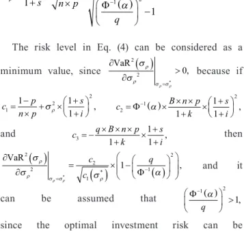
The risk level in Eq. (4) can be considered as a minimum value, since ^∂

( )

∂ >

=

VaR²

2σ 0

σ

ρ ρ σ_ρ σ_ρ^*

, because if

c p

n p

s i

1

2

1 1 2

= − 1

× + +

+



 



×

σ_ρ , c B n p

k

s i

2 1

2

1

= ( )× × × 1

+ × +

+



 



Φ− α ,

and _c ^{q B n p}

k

s i

3 1

1

= − × × × 1

+ × +

+ , then

∂

( )

∂ =

( )

^{× −}^^^ ^{( )}^^^



 



=

−

VaR²

2

1

1 2

σ 1

σ σ α

ρ

ρ σ_ρ σ_ρ^* ρ

*

c , c

q

Φ and it

can be assumed that ^^Φ⁻ ^{( )}

 

 >

1 2

α 1

q ,

since the optimal investment risk can be calculated only then if this condition is met.

It is worth noting that the optimal investment risk could only then be equal to zero when p = 1 or i = ˗1, but these two assumptions are not characteristic for many insurance types in practice. In case of the i value (the technical rate of return that is applied to calculating the insurance premium, that could also be interpreted as a "guaranteed return") it may be assumed that in practice i > 0.

The p value indicates the probability of the insurance event occurrence, thus p = 1 indicates a situation when it is sure that the insurance event occurs. As a result of these con- siderations, in the model it may be concluded that from the point of view of solvency it is not optimal for an insurance company to invest into risk-free assets. In the model, the optimal investment risk can be calculated if ^^Φ⁻^{( )}

 

 >

1 2

α 1

q .

The optimal investment risk level depends on several parameters in the model. Fig. 1 illustrates how the

investment risk (measured by σ_ρ) is related to the solvency measure VaR, and it also shows that the solvency optimizing investment risk can be different for various insurance portfolio sizes (B = 1, p = 0.05, i = 0, s = 0.1, k = 0.05, q = 1.25, r_a = 0, α = 0.995).

Fig. 1 also illustrates that the size of the insurance portfolio influences the solvency optimizing investment risk level. As Eq. (5) indicates, the optimal investment risk is smaller for an insurer with a larger insurance portfolio size, since ^∂

∂σ_ρ^* <

n 0.

∂

∂ = − × × +

+ × −

( )



 

 −

× ⁻

σ

α

ρ

*

n n p

i s

p

q 1

2

1 1

1

3 1 2

Φ (5)

As far as other parameters are concerned, the effect on the optimal investment risk is mixed. Similar to the results of Hieber et al. (2015), for a higher technical rate of return (i) the optimal investment risk is also higher.

The rationale for this result is straightforward: for a higher

"guaranteed" return a higher expected investment return is required, and it is associated with a higher investment risk level. The "solvency multiplier" (indicated by s) is related to the "available" capital that is assumed to be higher than the regulatory requirement in the model, an increase in this s value results in a smaller optimal investment risk.

For a higher probability of the insurance event occurrence (indicated by p in the model) the optimal investment risk is smaller. On the whole, the theoretical results suggest that for a relatively large insurance portfolio (when the number of insurance contracts is relatively large) the optimal investment risk may be close to the risk-free level. The close- ness of the risk-free level and the optimal investment risk depends on other features of the insurance portfolio.

It is also an interesting question, whether the solvency optimizing investment level can be achieved with the maximization of the expected profit value. In the presented model setting the maximization of the profit corresponds to the minimization of the expected value of the random variable in Eq. (1), and ^∂ ^{( )}

∂ = − × × ×

+ × +

+ <

E q B n p

k s

i η

σ_ρ 1

1

1 0, thus the conclusion arises that the expected profit maximizing and the solvency optimizing investment risk level is not the same in the model. This result could be different under other model assumptions, for example another assumption about the solvency ratio may contribute to change the result about the difference between the two optimum values.

However, despite the simplicity of the model assumptions, the result about a higher profit optimizing investment risk

Fig. 1 VaR for different portfolio sizes Source: own calculations

(6)

level may also highlight the potentially important effect of solvency regulation in the insurance sector.

4 Conclusions

Solvency regulation in the financial sector currently has a strong focus on risk measurement and the evaluation of risks. The Solvency II directive in the European Union outlines investment principles so that insurance companies should invest the assets in accordance with the prudent person principle (Directive 2009/138/EC, 2009).

Mathematically, in a theoretical model setting one of the definitions of prudency could be that the most prudent investment level corresponds to the solvency optimizing investment risk. This paper aims to find an answer to the question, whether the solvency optimizing investment risk level is equal to the risk-free level, or a certain extent of "search for yield" behaviour (that currently may be observed in practice in the protracted low interest rate environment) may be considered as optimal.

To explore the main research question of the paper, a theoretical model is constructed in which, similar to the Solvency II regulation, the solvency is measured by VaR, and it is also assumed that the investment risk and the

insurance risk are uncorrelated. The theoretical results of the paper suggest that under the model assumptions the optimal investment risk level is not zero, thus simple investment risk minimization does not optimize solvency.

However, it should also be noted that the size of the insurance portfolio (the number of insurance contracts) also strongly influences the theoretical results: for a relatively large insurance portfolio the optimal investment risk level may be relatively close to the risk-free level.

During the interpretation of the results it should be emphasized that the presented model is relatively simple, and does not fully capture the complexity of the operation of an insurance company in practice. However, the presented results may also provide interesting insights about investment risk management in insurance, for example the results highlight the potentially important role of the insurance portfolio size on optimal investment risk level.

There are several ways how the theoretical model could be developed, among other options an important direction for future research is the refinement of the assumptions about the relationship between the available solvency capital and the investment risk level.

References

Abdymomunov, A., Gerlach, J. (2014) "Stress testing interest rate risk exposure", Journal of Banking & Finance, 49, pp. 287–301.

https://doi.org/10.1016/j.jbankfin.2014.08.013

Albrecher, H., Bauer, D., Embrechts, P., Filipović, D., Koch-Medina, P., Korn, R., Loisel, S., Pelsser, A., Schiller, F., Schmeiser, H., Wagner, J. (2018) "Asset-liability management for long-term insurance business", European Actuarial Journal, 8(1), pp. 9–25.

https://doi.org/10.1007/s13385-018-0167-5

Albuquerque, R. (2012) "Skewness in Stock Returns: Reconciling the Evidence on Firm Versus Aggregate Returns", The Review of Financial Studies, 25(5), pp. 1630–1673.

https://doi.org/10.1093/rfs/hhr144

Bassetto, M., Cui, W. (2018) "The fiscal theory of the price level in a world of low interest rates", Journal of Economic Dynamics and Control, 89, pp. 5–22.

https://doi.org/10.1016/j.jedc.2018.01.006

Borio, C., Gambacorta, L. (2017) "Monetary policy and bank lending in a low interest rate environment: Diminishing effectiveness?", Journal of Macroeconomics, 54(B), pp. 217–231.

https://doi.org/10.1016/j.jmacro.2017.02.005

Bottero, M., Minoiu, C., Peydro, J. L., Polo, A., Presbitero, A. F., Sette, E. (2019) "Negative Monetary Policy Rates and Portfolio Rebalancing: Evidence from Credit Register Data", IMF Working Papers, International Monetary Fund, Working Paper No. 19/44. Available at: https://www.imf.org/en/Publications/

WP/Issues/2019/02/28/Negative-Monetary-Policy-Rates-and- Portfolio-Rebalancing-Evidence-from-Credit-Register-Data-46638 [Accessed: 29 July 2019]

Bouyé, E., Wang, T. (2015) "Dynamic Strategies for Net Income Generation in a Low Interest Rate Environment", Procedia Economics and Finance, 29, pp. 82–95.

https://doi.org/10.1016/S2212-5671(15)01115-6

Cociuba, S. E., Shukayev, M., Ueberfeldt, A. (2016) "Collateralized borrowing and risk taking at low interest rates", European Economic Review, 85, pp. 62–83.

https://doi.org/10.1016/j.euroecorev.2016.02.005

Consigli, G., Moriggia, V., Vitali, S., Mercuri, L. (2018) "Optimal insurance portfolios risk-adjusted performance through dynamic stochastic programming", Computational Management Science, 15(3), pp. 599–632.

https://doi.org/10.1007/s10287-018-0328-7

Dickson, D. C. M., Hardy, M. R., Waters, H. R. (2011) "Actuarial mathematics for life contingent risks", Cambridge University Press, Cambridge, UK.

Directive 2009/138/EC of the European Parliament and of the Council of 25 November 2009 on the taking-up and pursuit of the business of Insurance and Reinsurance (Solvency II) (recast), 2009. Official Journal of the European Union [online] L 335, pp. 1–155. Available at: https://eur-lex.europa.eu/legal-content/en/

ALL/?uri=CELEX%3A32009L0138 [Accessed: 29 July 2019]

Eisenberg, J., Krühner, P. (2018) "The impact of negative interest rates on optimal capital injections", Insurance: Mathematics and Economics, 82, pp. 1–10.

https://doi.org/10.1016/j.insmatheco.2018.06.004

(7)

Eling, M., Holder, S. (2013) "Maximum Technical Interest Rates in Life Insurance in Europe and the United States: An Overview and Comparison", The Geneva Papers on Risk an Insurance – Issues and Practice, 38(2), pp. 354–375.

https://doi.org/10.1057/gpp.2012.41

European Central Bank (2015) "Financial Stability Review", [pdf]

European Central Bank, Frankfurt, Germany. Available at: https://

www.ecb.europa.eu/pub/pdf/other/financialstabilityreview201511.

en.pdf [Accessed: 29 July 2019]

European Central Bank (2019) "Financial Stability Review", [pdf]

European Central Bank, Frankfurt, Germany. Available at: https://

www.ecb.europa.eu/pub/pdf/fsr/ecb.fsr201905~266e856634.

en.pdf [Accessed: 29 July 2019]

Fache Rousová, L., Giuzio, M. (2019) "Insurers' investment strategies: pro- or countercyclical?", European Central Bank Working Paper Series No 2299. Available at: https://www.ecb.europa.eu/pub/pdf/scpwps/

ecb.wp2299~1d060f6979.en.pdf [Accessed: 17 March 2020]

Fama, E. F., French, K. R. (2004) "The Capital Asset Pricing Model:

Theory and Evidence", Journal of Economic Perspectives, 18(3), pp. 25–46.

https://doi.org/10.1257/0895330042162430

Garín, J., Lester, R., Sims, E., Wolff, J. (2019) "Without looking closer, it may seem cheap: Low interest rates and government borrowing", Economics Letters, 180, pp. 28–32.

https://doi.org/10.1016/j.econlet.2019.02.024

Heider, F., Saidi, F., Schepens, G. (2018) "Life below zero: bank lending under negative policy rates", European Central Bank, Working Paper Series, No 2173. [online] Available at: https://www.ecb.europa.eu/

pub/pdf/scpwps/ecb.wp2173.en.pdf [Accessed: 29 July 2019]

Hieber, P., Korn, R., Scherer, M. (2015) "Analyzing the effect of low interest rates on the surplus participation of life insurance policies with different annual interest rate guarantees", European Actuarial Journal, 5(1), pp. 11–28.

https://doi.org/10.1007/s13385-014-0102-3

Holsboer, J. H. (2000) "The Impact of Low Interest Rates on Insurers", The Geneva Papers on Risk and Insurance – Issues and Practice, 25(1), pp. 38–58.

https://doi.org/10.1111/1468-0440.00047

Insurance Europe (2014) "Why insurers differ from banks", [pdf]

Insurance Europe, Brussels, Belgium. Available at: https://www.

insuranceeurope.eu/sites/default/files/attachments/Why%20insur- ers%20differ%20from%20banks.pdf [Accessed: 29 July 2019]

Jarrow, R. A. (2013) "The zero-lower bound on interest rates: Myth or reality?", Finance Research Letters, 10(4), pp. 151–156.

https://doi.org/10.1016/j.frl.2013.08.003

Jensen, T. K., Johnson, R. R., McNamara, M. J. (2019) "Funding conditions and insurance stock returns: Do insurance stocks really benefit from rising interest rate regimes?", Risk Management and Insurance Review, 22(4), pp. 367–391.

https://doi.org/10.1111/rmir.12133

Kablau, A., Weiß, M. (2014) "How is the low-interest-rate environment affecting the solvency of German life insurers?", Deutsche Bundesbank Discussion Paper No 27/2014.

Available at: https://www.bundesbank.de/resource/blob/624860/45a3e- c9158252e5e48d54b9f8b519ad2/mL/2014-10-27-dkp-27-data.pdf [Accessed: 17 March 2020]

Katahira, K., Chen, Y., Hashimoto, G., Okuda, H. (2019) "Development of an agent-based speculation game for higher reproducibility of financial stylized facts", Physica A: Statistical Mechanics and its Applications, 524, pp. 503–518.

https://doi.org/10.1016/j.physa.2019.04.157

Kurowski, Ł. K., Rogowicz, K. (2017) "Negative interest rates as sys- temic risk event", Finance Research Letters, 22, pp. 153–157.

Lagerås, A., Lindholm, M. (2016) "Issues with the Smith-Wilson method", Insurance: Mathematics and Economics 71, pp. 93–102.

Liang, Z., Zhao, X. (2016) "Optimal mean-variance efficiency of a family with life insurance under inflation risk", Insurance: Mathematics and Economics, 71, pp. 164–178.

Lintner, J. (1965) "The Valuation of Risk Assets and the Selection of Risky Investments in Stock Portfolios and Capital Budgets", The Review of Economics and Statistics, 47(1), pp. 13–37.

https://doi.org/10.2307/1924119

Löfvendahl, G., Yong, J. (2017) "Insurance supervisory strategies for a low interest rate environment", Bank for International Settlements, Financial Stability Institute, FSI Insights on policy implementa- tion No 4, Basel, Switzerland. Available at: https://www.bis.org/

fsi/publ/insights4.pdf [Accessed: 29 July 2019]

Lundblad, C. (2007) "The risk return tradeoff in the long run: 1836- 2003", Journal of Financial Economics, 85(1), pp. 123–150.

https://doi.org/10.1016/j.jfineco.2006.06.003

McNeil, A. J., Frey, R., Embrechts, P. (2005) "Quantitative Risk Management: Concepts, Techniques and Tools", Princeton University Press, Woodstock, UK.

Merton, R. C. (1980) "On estimating the expected return on the market.

An exploratory investigation", Journal of Financial Economics, 8(4), pp. 323–361.

https://doi.org/10.1016/0304-405x(80)90007-0

Mulvey, J. M., Madsen, C., Morin, F. (1999) "Linking strategic and tacti- cal planning systems for asset and liability management", Annals of Operations Research, 85, pp. 249–266.

https://doi.org/10.1023/A:1018925912190

Nucera, F., Lucas, A., Schaumburg, J., Schwaab, B. (2017) "Do negative interest rates make banks less safe?", Economics Letters, 159, pp. 112–115.

https://doi.org/10.1016/j.econlet.2017.07.014

Patel, J., Russo, V., Fabozzi, F. J. (2018) "Using the right implied volatility quotes in times of low interest rates: an empirical analysis across different currencies", Finance Research Letters, 25, pp. 196–201.

Schmeiser, H., Wagner, J. (2015) "A Proposal on How the Regulator Should Set Minimum Interest Rate Guarantees in Participating Life Insurance Contracts", The Journal of Risk and Insurance, 82(3), pp. 659–686.

https://doi.org/10.1111/jori.12036

Schmidli, H. (2015) "Extended Gerber-Shiu functions in a risk model with interest", Insurance: Mathematics and Economics, 61, pp. 271–275.

(8)

Sharpe, W. F. (1964) "Capital Asset Prices: A Theory of Market Equilibrium under Conditions of Risk", The Journal of Finance, 19(3), pp. 425–442.

https://doi.org/10.2307/2977928

Tsai, J. T., Wang, J. L., Tzeng, L. Y. (2010) "On the optimal product mix in life insurance companies using conditional value at risk", Insurance: Mathematics and Economics, 46(1), pp. 235–241.

Wang, J., Yang, M. (2013) "On the risk return relationship", Journal of Empirical Finance, 21, pp. 132–141.

https://doi.org/10.1016/j.jempfin.2013.01.001

Wang, X. (2016) "Catastrophe equity put options with target variance", Insurance: Mathematics and Economics, 71, pp. 79–86.