Vol.:(0123456789) ORIGINAL ARTICLE
Irrational risk‑taking of professionals? The relationship between risk exposures and previous profits
Edina Berlinger1 · Barbara Dömötör1 · Balázs Árpád Szűcs1
Accepted: 24 May 2021 / Published online: 11 June 2021
© The Author(s) 2021
Abstract
The risk attitude of investors is a key factor determining financial asset prices and market trends. Changes in risk attitude may be due to the interference of macro-level (business cycle) and micro-level (individual experience) effects. We investigate the impact of individual experience on the subsequent risk-taking attitude of profession- als via the analysis of the trading activity of 351 non-financial firms and (non-bank) financial institutions (insurance companies, financial intermediaries, etc.) covering 57,039 FX forward transactions in a highly volatile period between January 2008 and November 2012. Panel regressions for all firms and institutions do not show significant behavioral patterns. When investigating each client separately, however, we find that 39.7% of the clients having enough transactions to analyze statistically tend to increase their risk exposure irrationally after large gains or losses which can be the manifestation of the break-even and house-money effects well-documented in the literature for non-professionals. This irrational behavior may destroy value, so both market players and regulators should pay attention to monitor and control it.
Keywords Corporate risk management · Behavioral finance · Individual experience · Break-even effect · House-money effect
JEL Classification G02 · G11
* Barbara Dömötör
barbara.domotor@uni-corvinus.hu Edina Berlinger
edina.berlinger@uni-corvinus.hu Balázs Árpád Szűcs
balazsarpad.szucs@uni-corvinus.hu
1 Department of Finance, Corvinus University of Budapest, Fővám Square 8, Budapest 1093, Hungary
Introduction and literature review
The risk attitude of economic players affects risk premia, investment decisions, and asset prices (Benchimol 2014). This is especially true in the case of high- risk investments like innovative start-ups and emerging markets. Risk attitude is an important factor even in developed industries and countries as it may become endogenous and path-dependent, and positive feedback effects may lead to bub- bles and increased systemic risk.
Rational models of decision making assume that players are maximizing their utility function which is stable over time. Utility is usually a concave function of wealth, which implies risk-averse players. According to a large body of empirical and experimental literature, people tend to risk more dollars as they get richer, so their absolute risk aversion is decreasing in wealth (Tversky and Kahneman 1992). This is consistent with CRRA (constant relative risk aversion) utility func- tions, too, which are the most popular in economic literature (Arrow 1965; Mehra and Prescott 1985; Herings and Kubler 2007), implying that people keep a con- stant percentage of their portfolio in risky assets independently of their actual level of wealth. Therefore, in rational models with a CRRA utility function (in a stable environment), if the investor realizes a positive profit, his wealth increases, the percentage of risky assets remains constant, but the absolute value of the risky assets increases, so there is a positive relationship between previous profits and the subsequent absolute risk exposure. (We use the term „profit” as a signed number, a negative profit means a loss.)
Contrary to this, Goetzmann et al. (2007) demonstrated that rational players may be motivated to decrease (increase) their risk exposure after large random positive (negative) profits. They do so when they try to manipulate classical per- formance measures which build on the concept of risk-adjusted expected return (e.g., Sharpe-ratio). So, we have a rational explanation for the negative relation- ship between previous profits and risk-taking, too.
Beyond rationality, Minsky (1986) described a procyclical behavior of the investors implying a strong positive relationship between profits and risk-taking.
According to the financial instability hypothesis, people tend to take increasingly risky positions in a booming market, and when the bubble bursts, risk aversion increases dramatically, and market players start to deleverage their positions intensively. This Minsky-effect has three components: (i) investors remember less those events that happened long ago (recency effect), (ii) investors expect the trend to continue (momentum trading), (iii) previous positive profits increase risk- taking (experience-based risk-taking attitude).
Cohn et al. (2015) analyzed the behavior of financial market professionals on a hypothetical equity market with the help of a laboratory experiment and found a strong Minsky-effect: in a boom scenario, risk appetite increased while in a bust scenario, it decreased significantly. This effect helps to understand the building up and down of asset bubbles which contributes to the high volatility of finan- cial markets. Guiso et al. (2018) strengthened this by surveying the clients of an Italian bank and investigating their portfolio data. They found that after the
crisis of 2008, clients heavily divested stocks, which could not be explained on a rational basis, these decisions were rather emotionally driven. Mengel et al.
(2016) designed an experiment to analyze time-varying risk appetite at a micro- level focusing on the effects of individual experience. Participants of the experi- ment could choose between a risk-free investment and a lottery. It turned out that large uncertainty experienced in the past led to a decreased risk appetite. This result can provide a micro-level explanation for the Minsky-effect.
The prospect theory supported by a large amount of psychological experiments states that people evaluate the outcome of risky investments relative to a reference point which is not stable over time, their value function is concave for positive prof- its and convex for losses; moreover, they use subjective probabilities (Tversky and Kahneman 1979). These findings cannot be reconciled with utility maximization and result in a special fourfold pattern of risk-taking (Tversky and Kahneman 1992).
People are risk-averse when they expect to win with high probability (equity invest- ments) or to loose with low probabilities (insurance), and they are risk seeking when they expect to win with low probability (lottery) or to loose with high probability (break-even effect).
Post et al. (2008) analyzed the database of a TV show (Deal or no deal?) and found that people tended to risk more (less) after profits of large (small) absolute value. These findings were strengthened by laboratory experiments, as well. Post et al. (2008) concluded that people had difficulties to adapt to new situations, their reference point is sticky. After losing a lot, players tried to avoid loss realization at any cost, so they took irrationally large risk just to give themselves a chance to get back to the initial (zero-loss) position (break-even effect); and conversely, after win- ning a lot, they did not consider the gain as real, they thought it was still the money of the casino (the house) and risked it more easily in the spirit of „easy-come-easy- go” (house-money effect). Clearly, both break-even and house-money effects can be attributed to mental accounting problems. Note that an increasing risk appetite fol- lowing large positive profits can be attributed to other behavioral effects, as well, for example to the confirmation bias (searching for, interpreting, favoring, and recalling information in a way that confirms or supports one’s prior beliefs or values) or to overconfidence (when a person’s subjective confidence in his or her judgments is greater than the objective value of those judgments).
Interestingly, also professional traders seem to exhibit these irrational behavioral effects. Coval and Shumway (2005), for example, observed a strong intraday break- even effect on the US T-bonds’ futures market of the Chicago Board of Trade. They analyzed all transactions on the traders’ own account in 1998 and found that traders suffering loss in the morning session were 16% more likely to take above-the-aver- age risk in the afternoon. This effect did not prevail on a longer term, so the gains and losses had no further effect on the next day’s behavior. Also, Faulkender (2005) and Brown et al. (2006) showed that the hedging activity of corporations is domi- nated by behavioral effects, and it is characterized rather by myopic speculation than rational, text-book-style risk management.
In this paper, we investigate behavioral effects on risk-taking similarly to Post et al. (2008) but we focus on 351 non-financial firms and non-bank financial institu- tions (insurance companies, financial intermediaries, etc.), being the clients of the
Hungarian branch of ING Bank. We analyze their trading activity on the FX forward market. We can disregard the effects of the general market sentiment and can focus on the micro-level experience with previous profits because traders on the forward market can have both long and short positions, and we control for the general macro trends. However, our investment horizon is much longer than that of Post et al.
(2008) or Coval and Schumway (2005) who investigated intraday behavioral pat- terns, whereas we calculate profits and exposures on a monthly basis and run panel regression models with time and firm fixed effects. We find no general behavioral patterns characterizing the whole sample, which can be explained by the longer time horizon and/or the rationality of most of the professional traders.
In the next step, we analyze the behavior of the clients one by one on a daily basis. Profits are calculated as the exponentially weighted average of the previous year’s daily profits (giving more weight to the recent experience), and the risk expo- sure is the absolute value of the aggregate (gross or net) open positions at the end of the day denominated in Hungarian forint. We examine the relationship between previous profits (explanatory variable) and the subsequent risk exposure (depend- ent variable) with the help of multivariate OLS regression for each player where the control variable is the average FX position of the given player which is a proxy for its hedging need. Regressions are estimated separately for negative and positive profits. Regression coefficients are significant neither for negative nor for positive profits in the case of 48.2% of the clients. For 36.1% only one side is significant, and coefficients are significant for both sides only for 15.7% of the clients. However, when both sides are significant, a V-shape is dominant for 69.2% of these clients while the frequency of the other three possible shapes (/\, / /, \ \) altogether is only 30.8%.
Thus, the V-shape is a dominant pattern, which is consistent with the findings of Post et al. (2008) as it reflects that risk appetite increases after profits of large absolute value (break-even and house-money effects). Clearly, a V-shape cannot be explained by rational decision making or the Minsky-effect, because these would imply a monotonic relationship between profits and risk-taking. It is also notable that when only one leg is significant, then it is a half V-shape in 80.0% of the cases:
a negative coefficient on the negative side (53.3%) or a positive coefficient on the positive side (26.7%), which again can be the sign of the break-even and the house- money effects, respectively. All in all, 39.7% of the clients show a V-shape or a half V-shape pattern, which can be due to behavioral effects.
In “Data” section, we describe the database and the methods. In “General behav- ioral patterns” and “Client-level behavioral patterns” sections, general and client- level behavioral patterns are investigated, respectively. Finally, in “Conclusions”
section, we derive conclusions.
Data
We accessed a comprehensive database of all FX transactions of corporate and institutional (non-bank) clients of the Hungarian branch of ING Bank N. V. The database contains all FX-deals except the interbank transactions. The bank had
481 corporate and institutional (non-bank) clients between January 2, 2008 and November 3, 2012. The total number of transactions was 88,500. We received eight records for each transaction: client code (anonymous), sector code, deal date, value date, bought currency, bought amount, sold currency, and sold amount.
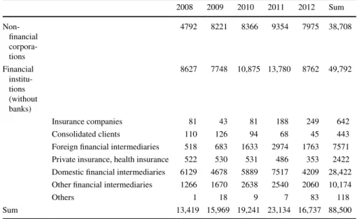
Around 44% of the transactions involved non-financial corporations; in the case of the remaining 56%, the trading partners were (non-bank) financial institu- tions, see Table 1.
The number of transactions was growing in this period, peaking in 2011. Note, however, that the last year—2012—was incomplete as data last until November.
Figure 1 shows the frequency of various currencies involved. (A transaction involves two currencies, therefore, frequencies in Fig. 1 sum up to 200%.)
Table 1 FX transaction numbers by year and client type
2008 2009 2010 2011 2012 Sum
Non-financial corpora- tions
4792 8221 8366 9354 7975 38,708
Financial institu- tions (without banks)
8627 7748 10,875 13,780 8762 49,792
Insurance companies 81 43 81 188 249 642
Consolidated clients 110 126 94 68 45 443
Foreign financial intermediaries 518 683 1633 2974 1763 7571 Private insurance, health insurance 522 530 531 486 353 2422 Domestic financial intermediaries 6129 4678 5889 7517 4209 28,422 Other financial intermediaries 1266 1670 2638 2540 2060 10,174
Others 1 18 9 7 83 118
Sum 13,419 15,969 19,241 23,134 16,737 88,500
0%
20%
40%
60%
80%
100%
Percentage in transacons
Currencies Fig. 1 Currencies involved in FX transactions
The Hungarian forint (HUF), the euro (EUR), and the US dollar (USD) were the most frequently traded currencies, these were involved in most of the transactions.
The difference between value date and deal date is the maturity of the deal. Figure 2 depicts the frequency of the different maturities in the observed transactions.
Frequencies are ordered to the minimum of the interval on the x-axis. For exam- ple, almost 20% of the transactions have a less than 1-month maturity (the maturity expressed in days is 0 to 30), and most of these are spot transactions. Most deals (around 60%) fall into the next category, their maturity is between 30 and 60 days.
After removing erroneous observations, spot deals, and non-HUF transactions, we have 57,151 transactions conducted with 351 different clients. The next step was to download daily FX rates between HUF and the other currencies from the webpage of the Hungarian National Bank (MNB). HUF rates for Slovak koruna, Hong Kong dollar, and South African rand are not available for the entire period, therefore, the 112 trans- actions where these currencies were involved are removed from the sample. So, finally, we get 351 clients and 57,039 transactions.
In the following, we specify how exposure and profit variables are calculated.
We do not have information about clients’ other positions, just their forward posi- tions at ING Bank, so their risk exposure cannot be measured in relative but only in absolute terms. First, we calculate the exposure Xi,t for the ith client on the tth day by aggregating the HUF value of his open positions in different currencies. As it is usual in risk management, exposures can be calculated either on a net or on a gross basis:
or
(1) Xi,t=Xnet
i,t =
||
||
||
∑
j
Fj,tQi,j,t
||
||
||
Xi,t=Xgrossi,t =∑ (2)
j
Fj,t|
||Qi,j,t|
||,
0%
10%
20%
30%
40%
50%
60%
70%
Fig. 2 Maturity of FX transactions (in days)
where Fj,t is the HUF spot daily mid-price of one unit of the jth foreign currency downloaded from the webpage of the Hungarian National Bank (MNB) and Qi,j,t is the net size of the open position of the ith client in the jth currency at the end of the tth day expressed in units of the foreign currency (positive if long and negative if short from the client’s perspective). Thus, the net and the gross exposures in (1) and (2) are non-negative numbers.
Then we determine the daily aggregate profit 𝜋i,t for each client i on each day t for all currencies j:
By (3), for the sake of simplicity, we disregard cross-currency interest rate differ- ences and suppose that profits come only from the change of FX rates. Note that 𝜋i,t does not equal the difference between forint values of the client exposure on con- secutive days, because we adjust for expired and freshly opened positions as well.
General behavioral patterns
We assume that the clients of ING Bank, that is traders sitting in corporate or financial institutions’ treasuries, take FX forward positions basically to hedge their initial FX positions coming from their core activities (export/import, ser- vice of their own clients, etc.). At the same time, however, clients may have some speculative positions as well.
Our research question is whether previous profits influence the subsequent risk exposure on the whole sample. First, to capture general patterns characterizing all clients in the sample (and to avoid too many zeros in the data table), we switch from a daily to a monthly scale:
where Dm is the number of trading days in month m. By using the monthly average values in the regression, we can avoid insignificant results due to missing data.
The first idea would be to estimate the following panel regression model:
where Xi,m is the average exposure of client i in month m and 𝜋i,m−1 is the average daily profit realized by client i in the previous month.
(3) 𝜋i,t=∑
j
Qi,j,t−1
( Fj,t Fj,t−1 −1
) .
(4) Xi,m=
∑Dm
t=1Xi,t Dm ,
(5) 𝜋i,m=
∑Dm t=1𝜋i,t
Dm ,
(6) Xi,m=𝛼i+𝛽𝜋i,m−1+𝜀i,m,
Clearly, (6) would be a misspecified model because an important variable influenc- ing both previous profits and present exposures is omitted, namely previous exposures.
The larger previous exposures were profits of larger absolute values could have been realized, and the present exposure is supposed to be larger, too. Assuming a stable busi- ness activity of the clients, previous exposures serve also as a proxy for the actual hedg- ing need.
To investigate the relationship between exposures and previous profits, we should look back in time for several months to capture the potential long-lasting effects, so we use four lagged values of the monthly profits. According to prospect theory, it is worth to differentiate between negative and positive profits, so we also apply the four lagged variables both for positive and negative monthly profits separately. Introducing a dummy variable for December, we also control for the increased activity of the trad- ers at the end of the year, which can be motivated by window-dressing (Lakonishok et al. 1991). Firm fixed effects ( 𝛼i ) account for differences in firms’ characteristics, and year dummies control for the macro trends (price movements, volatility, other macro conditions).
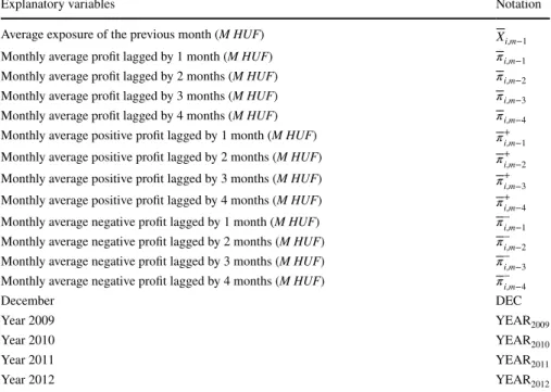
Explanatory variables in the panel regressions are summarized in Table 2.
So, the general form of the investigated panel regression model is specified as
(7) Xi,m=𝛼i+
∑4 k=1
𝛽k𝜋i,m−k+𝛿Xi,m−1+𝜃DEC+
2012∑
l=2009
𝜏lYEARl+𝜀i,m.
Table 2 Explanatory variables of the panel regression models
Explanatory variables Notation
Average exposure of the previous month (M HUF) X
i,m−1
Monthly average profit lagged by 1 month (M HUF) 𝜋i,m−1
Monthly average profit lagged by 2 months (M HUF) 𝜋i,m−2
Monthly average profit lagged by 3 months (M HUF) 𝜋i,m−3
Monthly average profit lagged by 4 months (M HUF) 𝜋i,m−4
Monthly average positive profit lagged by 1 month (M HUF) 𝜋+i,m−1 Monthly average positive profit lagged by 2 months (M HUF) 𝜋+i,m−2 Monthly average positive profit lagged by 3 months (M HUF) 𝜋+i,m−3 Monthly average positive profit lagged by 4 months (M HUF) 𝜋+i,m−4 Monthly average negative profit lagged by 1 month (M HUF) 𝜋−i,m−1 Monthly average negative profit lagged by 2 months (M HUF) 𝜋−i,m−2 Monthly average negative profit lagged by 3 months (M HUF) 𝜋−i,m−3 Monthly average negative profit lagged by 4 months (M HUF) 𝜋−i,m−4
December DEC
Year 2009 YEAR2009
Year 2010 YEAR2010
Year 2011 YEAR2011
Year 2012 YEAR2012
The dependent variable is the monthly average exposure, and the explanatory vari- ables are the profits of the last 4 months and the previous month’s exposure in Model 1.
Model 2 extends this model by involving the December-effect and year dummies.
In the next specifications, positive and negative profits are differentiated:
Models 3 and 4 involve positive profits and negative profits separately; while Model 5 contains both positive and negative profits as explanatory variables. We run panel regressions with cluster-robust standard error to account for heteroscedasticity and cor- relation in the error term within the clients. Table 3 shows the regression coefficients and their p-values. (In Table 3, we present results only with net exposures, gross expo- sures give similar results.)
Remark A positive coefficient means increasing risk-taking as a function of previ- ous profits in the ranges of both positive and negative profits. Note that profits are signed numbers. The benchmark year is 2008.
The exposure of the previous month is significant in all the specifications; the only other significant variable is the profit lagged by 2 months in Models 1 and 2, and the negative profit lagged by 2 and 3 months in Models 4 and 5. We can see from Fig. 2 that most of the transactions have a maturity of 1–2 months, so it can last several months for the clients to effectuate their trading strategy.
Most importantly, the signs of the coefficients of previous profits are positive both in the regions of negative and positive profits (where these are significant), which is con- sistent with a CRRA utility function. Behavioral effects could be detected only if profit coefficients were of different sign in different regions. We can conclude, therefore, that we find no signs of irrational risk-taking at this level of aggregation, which can be due to the rational behavior of most of the professional traders in the sample, at least on a monthly time scale. In the following, we investigate the client-level data to identify cli- ents with potential irrational behavior.
Client‑level behavioral patterns
For a more detailed, client-level analysis, we return to a daily time scale and specify two separate linear regression models for each client to explain their daily exposure, one for the region of negative and one for the region of positive profits:
(8) Xi,m=𝛼i+
∑4 k=1
𝛽k+𝜋+i,m−k+
∑4 k=1
𝛽k−𝜋−i,m−k+𝛿Xi,m−1+𝜃DEC+
2012∑
l=2009
𝜏lYEARl+𝜀i,m.
(9) Xi,t=𝛼−i +𝛽i−
∼
𝜋
−
i,t−1+𝛿−iX̃i,t−1+𝜀i,t,
(10) Xi,t=𝛼+i +𝛽i+
∼
𝜋
+
i,t−1+𝛿+iX̃i,t−1+𝜀i,t,
Table 3 Coefficients of the explanatory variables and their p-values Explanatory variablesModel 1Model 2Model 3Model 4Model 5 Xi,m−1
0.904** (0.000) 0.904** (0.000) 0.897** (0.000) 0.933** (0.000) 0.962** (0.000)
𝜋i,m−1 − 4.654 (0.223) − 4.631 (0.225) 𝜋i,m−2
17.146** (0.001) 17.146** (0.001)
𝜋i,m−3
9.576 (0.186) 9.571 (0.186)
𝜋i,m−4 − 1.693 (0.808) − 1.710 (0.806) 𝜋+ i,m−1 − 12.283 (0.356) − 16.279 (0.37) 𝜋+ i,m−2
11.881 (0.327)
− 7.353 (0.524) 𝜋+ i,m−3 − 1.336 (0.923) − 15.497 (0.225) 𝜋+ i,m−4
3.660 (0.862) 5.941 (0.774)
𝜋− i,m−1 − 0.937 (0.893)
4.444 (0.623)
𝜋− i,m−2
27.149** (0.000) 30.404** (0.000)
𝜋− i,m−3
17.073* (0.043) 19.365** (0.009)
𝜋− i,m−4 − 3.955 (0.484) − 7.38 (0.185) DEC − 22.0 (0.250) − 30.1 (0.136) − 15.7 (0.377) − 13.2 (0.475)
Table 3 (continued) Explanatory variablesModel 1Model 2Model 3Model 4Model 5 YEAR2009 − 22.4 (0.190) − 20.3 (0.208) − 21.0 (0.229) − 19.9 (0.255) YEAR2010 − 11.6 (0.645) − 8.3 (0.735) − 16.6 (0.499) − 20.4 (0.413) YEAR2011 − 23.8 (0.284) − 22.6 (0.246) − 26.2 (0.245) − 28.8 (0.161) YEAR2012 − 30.8 (0.25) − 27.9 (0.206) − 32.5 (0.179) − 33.2 (0.178) R2 within0.82060.82070.81570.82330.8245 R2 between0.99940.99940.99930.99940.9992 R2 overall0.91310.91310.91070.91400.9142 Number of observations18,95418,95418,95418,95418,954 *p < 5%; **p < 1%
where 𝜋∼
−
i,t−1 and 𝜋∼
+
i,t−1 are client-specific previous negative and positive profits, respectively, and X̃i,t−1 is the average size of previous exposures of the client. Note, however, that previous profits and exposures are modelled slightly differently here (∼
𝜋i,t−1,X̃i,t−1
) than in the panel regression models (
𝜋i,m−1,Xi,m−1
) . There, the time scale was 1 month and only the last 4 months’ profits and the last month’s exposure was considered as potential explanatory variables. Here, we switch to a daily time scale and the weighted average of profits and exposures of the whole last year are calculated to account for yearly cycles and for the recency effect.
As we are looking for longer term behavioral effects, we take all profits in the last year into account but conferring more weights to more recent experiences:
Assuming 250 trading days per year, we use an exponential weighting function:
where Wk stands for the weight of the kth observation, k=1 is the oldest and k=250 is the most recent one, and
In this setting, the ratio between the largest and the smallest weight is around 245, meaning that the profit of yesterday is 245 times more important than that of a year ago. The last day’s weight is about 2.2% and the weight of the last 4 months is more than 85%.
The average exposures of the last year X̃i,t−1 is a control variable representing the actual hedging need. Just like in the case of previous profits, we use exponen- tial weights:
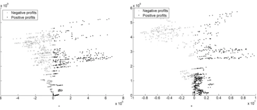
To detect client-level behavioral patterns, we estimate the coefficients of (9) and (10) for the trading data of the clients with the help of OLS regression. We allow clients to have different decision rules for previous negative and positive profits. To this end, we separate the samples of each client into two categories:
one where 𝜋∼i,t was negative, and another one where it was non-negative, see Fig. 3 showing the relationship between previous profits and present risk expo- sure of two selected clients.
Naturally, the lengths of the data series for different clients are not the same.
Some have open positions for the entire observation period, while others only for a very short time. Additionally, in some cases, these short series of open positions (11)
∼
𝜋i,t=∑
k
Wk⋅𝜋i,k.
(12) Wk= 1
A ⋅e−
k 250ln
( 1 250
)
,
(13) A=
∑250 i=1
e−
i 250⋅ln( 1
250
)
.
̃ (14) Xi,t−1=∑
k
Wk⋅Xi,k.
occur during the first year of the observation period which are lost for the regres- sion analysis, because of the exponentially weighted variables.
Coefficients in (9) and (10) are estimated first for the net exposure (1) and second for the gross exposure (2). Similarly to the aggregate model, results here are similar for net and gross exposure, so we present the results only for the net exposure (
Xnet
i,t
) . The primary focus of our attention is on the significance and the sign of the coeffi- cients of previous profits, 𝛽i− and 𝛽i+.
We consider a coefficient significant if it is significant at 95%, and the 𝜀 error term of the equation does not have a unit root according to the ADF (Augmented Dicky Fuller) test with 95% significance. There are three different cases for each coefficient:
– significant with positive sign (/) – significant with negative sign (\)
– not significant, so the sign does not matter (–)
Considering both negative and positive profits, a client’s behavior may have nine patterns. If coefficients are significant in both regressions, then the exposure as a function of the previous profits (see Fig. 3) may be:
– increasing for negative profits, increasing for positive profits (//-shape) – increasing for negative profits, decreasing for positive profits (/\-shape) – decreasing for negative profits, increasing for positive profits (\/-shape) – decreasing for negative profits, decreasing for positive profits (\\-shape)
There are four other patterns where one of the coefficients is not significant, and it is also possible that neither of the coefficients are significant. Table 4 summarizes all the nine behavioral patterns and their frequency in our data sample.
Monotone increasing behavioral patterns (1, 5, and 7) can be explained by rational decision making supposing for example a CRRA (constant relative risk aversion) utility function, or by the irrational Minsky-effect. Monotone decreasing
Fig. 3 Risk exposure as a function of previous profits for two selected clients
behavioral patterns (4, 6, and 8) can be explained rationally by a special utility func- tion or by the manipulation of the performance measures. Non-monotone behavio- ral patterns (2 and 3), however, cannot be explained rationally (supposing a stable wealth utility function), these would reflect irrational behavioral effects. Most of all, the V-shape pattern (3) is consistent with the findings of Post et al. (2008) which can be explained by the break-even effect (for negative profits) and the house-money effect (for positive profits) or by the confirmation bias to some extent.
Our research design is different from that of Post et al. (2008) in many aspects (long term versus intraday behavioral effects, professional versus non-professional decision makers, continuous versus discrete variables of profits and exposures), but we got very similar results in the sense that V-shape seems to be the dominant pat- tern (at least when we have any pattern) even if it is much less accentuated in our sample.
We can see in Table 4 that only 26 (15.7%) of the clients show significant patterns both for negative and positive profits. 18 of them (69%) exhibit a V-shape behavioral pattern which amounts to the 10.8% of the total number of clients included in the examination. Clients with pattern 3 tend to transact more frequently than the others but the average size of their open positions is relatively low.
Although we have a total of 351 clients in our sample, the number of clients displayed in Table 4 is 166. This is because we present only those clients that had enough transactions to perform all the tests for both negative and positive profits (at least 10 observations are needed to perform the test in our setting). So, we excluded 185 clients for the scarcity of data. Moreover, some of the remaining clients are excessively asymmetric in their profitability, meaning that they are either winning or losing most of the time and therefore, they have only few observations on the opposite side.
Note that patterns 6 and 7 may represent one half (left or right) of the V-shape, with no significant coefficient on the other side. These cases comprised 32 and 16 clients, respectively, which add up to 19.3% and 9.6% of the total number of clients.
Table 4 Behavioral patterns of the clients
# Behavioral patterns Number
of clients Percentage Average number of
transactions per client Average daily net exposure (M HUF)
1 pos_pos /, / 2 1.2 312 1030
2 pos_neg /, \ 0 0.0 n/a n/a
3 neg_pos \, / 18 10.8 618 1850
4 neg_neg \, \ 6 3.6 690 5750
5 pos_not /, – 1 0.6 409 2240
6 neg_not \, – 32 19.3 462 2600
7 not_pos –, / 16 9.6 459 3170
8 not_neg –, \ 11 6.6 543 2990
9 not_not –, – 80 48.2 206 1770
Overall 166 100.0
Focusing on this V-shape, Table 5 presents the same findings in a compressed form. It shows that significant cases consistent with V-shape altogether amount to 10.8% + 28.9% = 39.7% of the clients, while all the non-related significant cases add up to 12.0%. The remaining 48.2% of the clients do not exhibit significant coeffi- cients on either side.
We can conclude that a considerable percentage (51.8%) of the clients in our sam- ple (consciously or unconsciously) consider previous profits when deciding about their risk exposure. The V-shape pattern (10.8% of the clients) cannot be explained on a rational basis and it corresponds to the findings of Post et al. (2008), but here, with longer horizon and professional decision makers, it is less accentuated.
Of course, banks have more information, so they can investigate their clients’
behavior in more detail and develop more sophisticated models. In any case, those clients showing signs of irrational risk-taking should be monitored more carefully.
Conclusions
We investigate the risk-taking behavior of professional clients and find no behavio- ral patterns at an aggregate level. However, at a client level, 51.8% of the observed clients (having enough transactions to derive conclusions in statistical terms) show some significant relationship between previous profits and subsequent risk expo- sure. If there is a significant relationship, then the most representative pattern is V-shaped or half V-shaped. Therefore, 39.7% of the observed clients tend to increase (decrease) their exposures after profits of large (small) absolute value. A V-shape pattern cannot be explained by rational decision making and can be a sign of behav- ioral effects such as break-even and house-money effects similarly to the findings of Post et al. (2008).
As irrational behavioral effects destroy value both at individual and social lev- els, investors and regulators should pay attention to these symptoms. Our research has some obvious limitations as we had no information about clients’ actual hedg- ing need, their trading activities with other banks, the identity of their traders; and we had no mark-to-market forward prices when estimating profits. However, if this additional information is available, the methodology presented in this paper can be improved and used to detect market players exhibiting irrational behavior more effectively.
Table 5 Major behavioral
patterns # Behavioral patterns Number of
clients Percentage
a V-shape 18 10.8
b Half V-shape 48 28.9
c Other significant cases 20 12.0
d Nothing is significant 80 48.2
Overall 166 100.0
Acknowledgements This research was supported by the Higher Education Institutional Excellence Pro- gram of the Ministry for Innovation and Technology in the framework of the „Financial and Public Ser- vices” Research Project (Reference Number NKFIH-1163-10/2019) at Corvinus University of Budapest.
The authors are grateful for ING Bank N. V. for the database.
Funding Open access funding provided by Corvinus University of Budapest.
Declarations
Conflict of interest On behalf of all authors, the corresponding author states that there is no conflict of interest.
Open Access This article is licensed under a Creative Commons Attribution 4.0 International License, which permits use, sharing, adaptation, distribution and reproduction in any medium or format, as long as you give appropriate credit to the original author(s) and the source, provide a link to the Creative Com- mons licence, and indicate if changes were made. The images or other third party material in this article are included in the article’s Creative Commons licence, unless indicated otherwise in a credit line to the material. If material is not included in the article’s Creative Commons licence and your intended use is not permitted by statutory regulation or exceeds the permitted use, you will need to obtain permission directly from the copyright holder. To view a copy of this licence, visit http:// creat iveco mmons. org/ licen ses/ by/4. 0/.
References
Arrow, K.J. 1965. Aspects of the Theory of Risk-Bearing. Helsinki: Yrjö Jahnssonin Säätiö.
Benchimol, J. 2014. Risk aversion in the Eurozone. Research in Economics 68 (1): 39–56.
Brown, G., P. Crabb, and D. Haushalter. 2006. Are firms successful at selective hedging? The Journal of Business 79: 2925–2950.
Cohn, A., J. Engelmann, E. Fehr, and M.A. Maréchal. 2015. Evidence for countercyclical risk aversion:
An experiment with financial professionals. American Economic Review 105 (2): 860–885.
Coval, J.D., and T. Shumway. 2005. Do behavioral biases affect prices? The Journal of Finance 60 (1):
1–34.
Faulkender, M. 2005. Hedging or market timing? Selecting the interest rate exposure of corporate debt.
Journal of Finance 60: 931–962.
Herings, P.J.J., and F. Kubler. 2007. Approximate CAPM when preferences are CRRA. Computational Economics 29: 13–31.
Goetzmann, W., J. Ingersoll, M. Spiegel, and I. Welch. 2007. Portfolio performance manipulation and manipulation-proof performance measures. Review of Financial Studies 20 (5): 1503–1546.
Guiso, L., P. Sapienza, and L. Zingales. 2018. Time varying risk aversion. Journal of Financial Econom- ics 128 (3): 403–421.
Lakonishok, J., A. Shleifer, R. Thaler, and R. Vishny. 1991. Window dressing by pension fund managers.
The American Economic Review 81 (2): 227–231.
Mehra, R., and E.C. Prescott. 1985. The equity premium, a puzzle. Journal of Monetary Economics 15:
145–161.
Mengel, F., E. Tsakas, and A. Vostroknutov. 2016. Past experience of uncertainty affects risk aversion.
Experimental Economics 19: 151–176.
Minsky, H.P. 1986. Stabilizing an unstable economy. New Haven: Yale University Press.
Post, T., M.J. Van den Assem, G. Baltussen, and R.H. Thaler. 2008. Deal or no deal? Decision making under risk in a large-payoff game show. The American Economic Review 98 (1): 38–71.
Tversky, A., and D. Kahneman. 1979. Prospect theory: An analysis of decision under risk. Econometrica 47: 507–608.
Tversky, A., and D. Kahneman. 1992. Advances in prospect theory: Cumulative representation of uncer- tainty. Journal of Risk and Uncertainty 5: 297–323.
Publisher’s Note Springer Nature remains neutral with regard to jurisdictional claims in published maps and institutional affiliations.