Inventory investment and sectoral characteristics in some OECD countries

www.elsevier.com/locate/ijpe

Author’s Accepted Manuscript

Inventory investment and sectoral characteristics in some OECD countries

Attila Chikán, Erzsébet Kovács, Zsolt Matyusz

PII: S0925-5273(10)00294-X

DOI: doi:10.1016/j.ijpe.2010.08.005

Reference: PROECO 4514

To appear in:

Received date: 15 September 2008 Accepted date: 3 August 2010

Cite this article as: Attila Chikán, Erzsébet Kovács and Zsolt Matyusz, Inventory investment and sectoral characteristics in some OECD countries,

This is a PDF file of an unedited manuscript that has been accepted for publication. As

a service to our customers we are providing this early version of the manuscript. The

manuscript will undergo copyediting, typesetting, and review of the resulting galley proof

before it is published in its final citable form. Please note that during the production process

errors may be discovered which could affect the content, and all legal disclaimers that apply

to the journal pertain.

INVENTORY INVESTMENT AND SECTORAL CHARACTERISTICS IN SOME OECD COUNTRIES   

Attila Chikán*

Corvinus University of Budapest 1093 Budapest, Fővám tér 8. Hungary email: chikan@uni-corvinus.hu Erzsébet Kovács

Corvinus University of Budapest 1093 Budapest, Fővám tér 8. Hungary email: erzsebet.kovacs@uni-corvinus.hu Zsolt Matyusz

Corvinus University of Budapest 1093 Budapest, Fővám tér 8. Hungary email: zsolt.matyusz@uni-corvinus.hu  

Abstract 

This paper discusses the effects of sectoral structure on the long run macroeconomic  inventory behaviour of national economies. Data on fifteen OECD countries are included in  the analysis, which is based on correlation and cluster analysis methodologies. The study is  part of a long‐term research project exploring factors influencing the inventory behaviour of  national economies. 

First, we introduce some basic characteristics of macroeconomic inventory formation in the  fifteen OECD countries. We argue that our previous results on the existence of specific  characteristic features of macroeconomic inventory investment are justified, so it makes  sense to study the factors influencing those features. We then examine the contribution of  various sectors to the production of Gross Value Added in the countries involved and the  relationship between sectoral structure and inventory intensity (annual inventory change  /Gross Value Added). We find that the high share of agriculture and manufacturing increases  inventory intensity, that the increasing share of services has a negative effect and that the  role of construction and trade is not obvious. The relatively low stability of the statistical  results warns us to be cautious with our judgements. Further, case‐by‐case analysis would  be required to obtain more solid results. 

Keywords 

national inventories, inventory investment, Gross Value Added, macroeconomic factors,  sectoral structure 

INVENTORY INVESTMENT AND SECTORAL CHARACTERISTICS IN SOME OECD COUNTRIES   

Attila Chikán – Erzsébet Kovács – Zsolt Matyusz  Corvinus University of Budapest 

Introduction   

Our paper focuses on some macroeconomic characteristics of the inventory behaviour of  national economies. This research field is largely unexplored. There is only one country in  which it is adequately studied: the United States, from which a rich set of research results is  available (for some recent studies, see Ehemann, 2004, Hirsch, 1996, Humphreys, 2001,  Humphreys et al., 2001, Irvine, 2003a, Irvine, 2003b, Irvine, 2005, Irvine‐Schuh, 2005, Stern,  2001). There are very few country‐specific studies (for exceptions, see Dimelis−Lyriotaki,  2007, Guariglia−Mateut, 2010) and, as logically follows, there are very few cross‐country or  USA‐EU comparisons (Dimelis, 2001, West, 2002). It should be noted, however, that there  are interesting and recurring debates about the macroeconomic roles of inventories,  especially in connection with business cycles (see Blinder−Maccini, 1991, Lovell, 1994,  Chikán‐Milne‐Sprague, 1994, Dimelis, 2001 or Malgarini, 2007). 

Our interest in macroeconomic inventory behaviour dates back to the 1980s. At the First  International Symposium on Inventories in 1980, a paper on the effect of the general state  of the economy on inventory investment and structure was presented (Chikán, 1981). Since  that time,  we  have largely  focused  on  international  comparisons of  macroeconomic  inventory behaviour. As in the paper by Chikán−Horváth, 1999, we compared trends in 88  countries  to  determine  the  connection  between  the  inventory  intensity  (inventory  investment/GDP) of the individual countries and various components of GDP. The current  series of papers began in 2003 (Chikán−Tátrai, 2003), when we started to examine data from  14 OECD countries. (The data are probably the most reliable inventory data available). Since  that time, we have used the annual inventory investment/GDP ratio to measure national  inventory intensity. In the 2003 paper, we analysed the ratio’s relationship with various  measures and the development, growth and fluctuation of GDP. In our research, we have  used regression analyses and multivariable statistical methods. We have examined almost  twenty hypothesis and found interesting results, such as the following:  

− Inventories relative to GDP tend to decrease in developed countries after the  early 1980s; 

− The inventory characteristics of developed countries converge; 

− However, no general regression model that uses components of GDP usage  (fixed capital investment, exports, etc.) as independent variables can be found to  describe the inventory behaviour of various countries; 

− Even though the tendency of the inventory/GDP ratio to decrease and converge  appears to be valid across countries, the reasons for this tendency appear to  vary not only by country but also by time period 

In this paper, a new dimension of the factors that influence inventory investments is  analysed: the sectoral structure of the economy. 

In recent years, we have conducted a series of examinations of macroeconomic inventory  behaviour using multivariate statistical methods. Results of our research (the special  characteristics of which are methodological: we consequently use multivariate statistical  methods) have been reported in a series of papers presented at the biannual symposia of  the International Society for Inventory Research (ISIR). For the latest paper in the series,  with references to earlier papers, see Chikán‐Kovács, 2009. 

In this paper, we continue in the same methodological tradition, but take a different  perspective in our analysis: in earlier papers, we analysed national inventory behaviour in  terms of output (GDP use), but we now turn to input for our analysis (GDP production). We  take steps to understand the relationship between the sectoral structure of various  economies and their inventory behaviour. As stated earlier, we used OECD data for the  analysis—this  is the relatively richest  and  most  coherent  international database  for  macroeconomic inventory analysis. Even this database has limitations, however, which  restricted our options during the analysis. 

We believe we have obtained some interesting results even though several of our attempts  to find relationships between various sectoral characteristics of the studied economies and  their inventories have failed.  

Our main hypothesis is that the sectoral structure of economies and changes in this  structure influence inventory investments. We test this hypothesis by examining the  relationship between the sectoral structure and inventories from various angles. 

1. Characteristics of inventory investment in developed countries 

The starting point of our analysis was to examine inventory investments in OECD countries  where appropriate data were available. The focus of our study is the relative inventory  investment, i.e., the proportion of change in inventory level in a given year compared to the  Gross Value Added (GVA) of the country in the same year. We wanted to know whether  there is a relationship between this figure (which reflects the proportion of GVA invested in  inventories in any given year) and the sectoral structure of the economy (measured by the  contribution of various sectors to the production of GVA). The relative inventory investment  ratio (IC/GVA=inventory change/Gross Value Added) is positive in the case of increasing  inventory and negative in the case of inventory disinvestment. 

We had a nearly complete time series of the IC/GVA ratio of fifteen countries from among  the most developed economies of the world for the 1987‐2007 time period. (There are a few  countries for which the time series is a bit shorter, but even for these countries, the time  series are no smaller than seventeen subsequent years, a length that is adequate for our  analysis.) 

It must be mentioned here that, considering the high volatility of inventories, the use of data  that is more disaggregated, e.g., a quarterly time series, would greatly increase the  importance of our results. Such data are, unfortunately, unavailable in any international data  systems, so we had to compromise with annual data.  

However, this is not a major problem for our research because we are interested in long‐

term trends and aggregate behaviour. In fact, registering quarterly movements might have  detracted from the long‐term view of our work. Therefore, the use of annual data is both a  necessity (due to the lack of more frequent registering of inventories in national and  international statistics) and an advantage (making it necessary and possible to focus on  lasting effects).  

Figure 1.  Changes in inventory per Gross Value Added (%) 1987‐2007 

Figure 1 shows the graph of the IC/GVA ratio of all fifteen countries. It can be seen that  although the IC/GVA ratio varies substantially by year in each country, the changes remain in  a well‐definable range that shows a tendency of getting narrower over time. This is an  illustration of the tendency that we discussed in an earlier paper (Chikán et al 2005); namely,  that in every country, there exists a kind of “normal” level of inventories around which the  annual data fluctuate (for an explanation of such norms, see Kornai, 1980). It is a very  interesting discovery that these norms seem to converge in the developed countries. It is  also noteworthy that these normal levels have no clear tendency towards decline despite  the much‐celebrated improvements in companies’ inventory management. It appears that  the analysis in Chikán (1994) still holds true.   

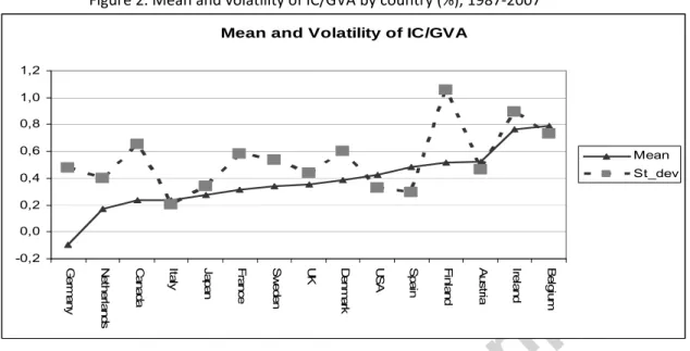
Figure 2 shows the long‐term averages (the “norms”) of the individual countries and their  volatility over the 21 years in the sample. Countries in the figure are arranged in an  increasing order of IC/GVA. There are no outliers. Only Germany had a negative average,  which was due to its serial inventory disinvestments in the new millennium. The total range  of the IC/GVA ratios is .884 (excluding Germany, .615) The overall average is .382, which can  be considered the median value as well. The variance was relatively low in Italy, Japan, the  USA and Spain, and relatively high in Finland, Ireland and Belgium.  

Figure 2. Mean and volatility of IC/GVA by country (%), 1987‐2007  

Mean and Volatility of IC/GVA

-0,2 0,0 0,2 0,4 0,6 0,8 1,0 1,2

Germany Netherlands Canada Italy Japan France Sweden UK Denmark USA Spain Finland Austria Ireland Belgium

Mean St_dev

We have examined the yearwise averages as well. Figure 3 shows the mean and the volatility  of the IC/GVA data of the 15 countries annually in graphical form. The averages fluctuate  (the range is between  ‐.26 and .84, so the averages are rather small). The annual range is  rather steady, with the exception of a few years in the early 1990s, when it was substantially  higher. The overall picture supports our opinion that developed countries’ inventory  investment norms are similar. 

Figure 3. Mean and volatility of the IC/GVA ratio by years, 1987‐2003. 

Volatility of IC/GVA

-0,4%

-0,2%

0,0%

0,2%

0,4%

0,6%

0,8%

1,0%

1987 1988 1989 1990 1991 1992 1993 1994 1995 1996 1997 1998 1999 2000 2001 2002 2003 2004 2005 2006 2007

year

mean stdev

2. Sectoral structure and inventory intensity 

Next, we analysed the sectoral structure of the fifteen countries in terms of the various  sectors’ contribution to the Gross Value Added. For the analysis, we first selected five  sectors: agriculture, manufacturing, construction, trade (wholesale + retail) and services.  

We  then  selected  six  subsectors  from  the  manufacturing  industry:  food,  chemicals, 

metallurgy, machinery, electronics and transport vehicles. The detailed results are shown in  tables in Appendix 1 and 2. Countries are sorted by their average IC/GVA ratios in ascending  order. We assigned two different values to each country. The first row (1987‐2003) shows  the long‐term average contribution of that industry to the country’s Gross Value Added. The  second row (Change) shows the ratio of the last five years’ (1999‐2003) contribution and the  first five years’ (1987‐1991) contribution to Gross Value Added. These ratios provide insight  to the dynamics of structural processes: we can see how the importance of certain industries  changed during the period of our investigation. For example, at the end of the period, the  contribution of agriculture to Gross Value Added in Germany was 78% of the contribution at  the beginning of the investigated period. 

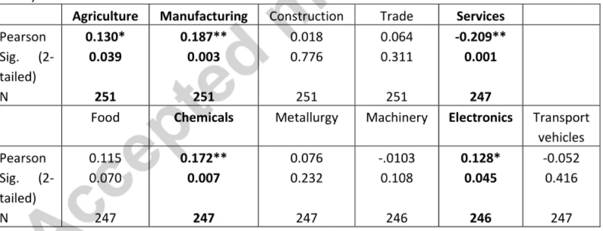
We examined the relationship between inventory intensity (the IC/GVA ratio) and the  sectoral structure of the 15 countries in the period of 1987‐2003 with a correlation analysis. 

As inventories constantly  increased during the past 20 years on average, a positive  significant correlation between certain industries’ structure and the IC/GVA ratio would  suggest that these industries are more intensive in terms of inventories. We analysed this in  two  steps.  First,  we  analysed  the  major  industries  of  agriculture,  manufacturing,  construction, trade and services. In the second step, we looked at certain manufacturing  sub‐industries, namely food, chemicals, metallurgy, machinery, electronics and transport  vehicles. 

The results of the correlation analysis between the annual proportion of various sectors’ 

contribution to GVA and countries’ IC/GVA ratio can be seen in Table 1.  

Table 1. Correlations between the IC/GVA ratio and sectoral structure (15 countries, 1987‐

2003) 

  Agriculture  Manufacturing  Construction  Trade  Services    Pearson 

Sig.  (2‐

tailed)  N 

0.130* 

0.039    251 

0.187** 

0.003    251 

0.018  0.776 

  251 

0.064  0.311 

  251 

‐0.209** 

0.001    247 

  Food  Chemicals  Metallurgy  Machinery  Electronics  Transport  vehicles  Pearson 

Sig.  (2‐

tailed)  N 

0.115  0.070 

  247 

0.172** 

0.007    247 

0.076  0.232 

  247 

‐.0103  0.108 

  246 

0.128* 

0.045    246 

‐0.052  0.416 

  247 

* Correlation is significant at the 0.05 level (2‐tailed) 

** Correlation is significant at the 0.01 level (2‐tailed)   

Unfortunately, even the significant correlations are not very strong. This can be explained by  the different nature of volatility of the two sets of data. While the sectoral structure does  not change rapidly in the short term, but instead changes incrementally, the IC/GVA ratio  may show greater yearly differences and one can find visible trends only in the long run. 

Nevertheless,  these  results  suggest  that  the  main  industries  of  manufacturing  and  agriculture  are  prime  candidates  for  differences  in  inventory  intensity.  From  the  manufacturing sub‐industries, the chemicals and electronics industries seem to be the most  important. Not surprisingly, the services industry correlates significantly and negatively with  the IC/GVA ratio.  

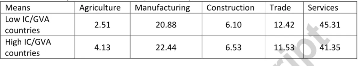
If one compares the contribution of various main sectors to the production of GVA in the  first and last five countries in the table in Appendix 1 (i.e., the least and most inventory‐

intensive national economies), the following observations can be made. In those countries  where the IC/GVA ratio is low, 

- the contribution of manufacturing, agriculture and construction to the GVA is  relatively lower, and 

- the proportion of services and trade is relatively higher than in the countries with  the highest IC/GVA ratios. See Table 2 for a summary. 

Table 2. Average contribution of the main industries to GVA (the five least and five most  inventory‐intensive countries, 1987‐2003) 

Means  Agriculture  Manufacturing Construction Trade  Services  Low IC/GVA 

countries  2.51  20.88  6.10  12.42  45.31 

High IC/GVA 

countries  4.13  22.44  6.53  11.53  41.35 

This  indicates  that  manufacturing,  agriculture  and  construction  are  generally  more  inventory‐intensive than trade and services. We believe that the relatively higher proportion  of trade in the low‐inventory countries may also be a consequence of the favourable overall  effects of a more extended trade sector on the economy. 

If we further analyse the long‐term contribution of the various sectors to the GVA by year,  we  can  say  that,  in  accordance  with  our  expectations,  the  overall  contribution  of  manufacturing, construction and agriculture (the inventory‐intensive sectors) to the GVA  decreases over time. For more details, see the tables in Appendix 3 and 4 at the end of the  article. An important explanation for these trends is the dramatic growth of the service  sector, the inventory intensity of which is fundamentally lower than that of other sectors. It  should be added that the country‐wise range of the proportion of the various sectors under  examination either decreases substantially (in the case of agriculture and construction) or  stagnates (in the case of trade and manufacturing—though the latter seems to increase  slightly in the last few years). This phenomenon supports our hypothesis on the decreasing  differences between the “inventory norms” of developed countries.  

3. Cluster analysis of sectoral effects   

We have executed cluster analysis of the fifteen countries to examine the common  characteristics of those countries that have a similar sectoral structure in given years. We  put over 300 items of data (on 17 countries for 21 years) into the space of the four main  sectors  that  we  considered  most  important  for  inventory  investment:  agriculture,  manufacturing, construction and trade. (Services were excluded because their share of total  inventories is very low). We used a Two‐Step Cluster Analysis procedure, which has very  favourable characteristics for our purposes. It is an exploratory tool designed to reveal  natural groupings (or clusters) within a dataset that would otherwise not be apparent. The  algorithm employed by this procedure has several desirable features that differentiate it  from traditional clustering techniques.¹ 

1 ‐ Handling of categorical and continuous variables: By assuming variables to be independent, a joint multinomial‐normal  distribution can be placed on categorical and continuous variables.  

After running the cluster analysis, we obtain four clusters of more or less the same size. They  contain 80% of the data in our database. Table 3 shows the cluster characteristics. 

Table 3. Cluster characteristics   

Cluster Distribution 

  N  % of Combined  % of Total 

Cluster 1  67  26.4%  21.3% 

Cluster 2  71  28.0%  22.5% 

Cluster 3  60  23.6%  19.0% 

Cluster 4  56  22.0%  17.8% 

Combined  254  100.0%  80.6% 

Excluded Cases  61    19.4% 

Total  315    100.0% 

Table 4. Cluster centroids   

  AGRICULTURE  TRADE  CONSTRUCTION  MANUFACTURING  MEAN  STD 

DEV 

MEAN  STD  DEV 

MEAN  STD  DEV 

MEAN  STD  DEV  CLUSTER  1  4.31  2.43  11.92  1.35  6.19  1.16  22.89  3.77 

  2  2.74  1.13  12.00  1.37  5.89  1.35  19.95  3.08 

  3  2.17  0.86  11.52  1.28  5.80  1.40  19.72  4.67    4  2.72  1.07  12.01  1.38  5.58  1.31  19.85  2.30    COMBINED  3.02  1.72  11.87  1.35  5.88  1.31  20.65  3.79 

Table 4 shows the cluster centroids. In general, the clusters look very similar, though we can  find some distinct characteristics. Cluster 1 members have the highest shares in the  agriculture, construction and manufacturing industries, while trade seems to be average. 

Cluster 2 members are average in all main industries. Cluster 3 members have below‐

average shares in agriculture and trade. Cluster 4 members are almost identical to Cluster 2  members, aside from the lower share in construction. 

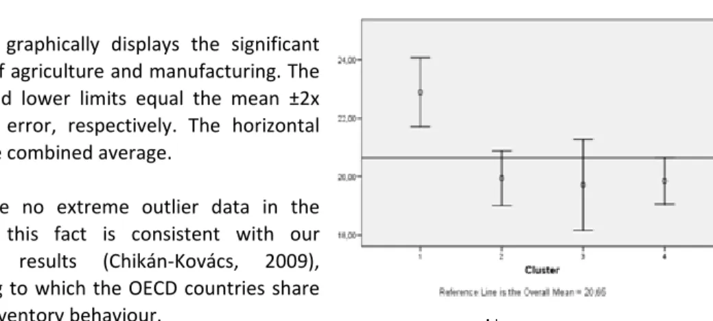
For stronger statistical support, we conducted one‐way ANOVA analysis to determine which  industries are significantly different in the clusters. We found that the two industries that  are significantly different in the four clusters are agriculture and manufacturing, so Cluster 1  members have an above‐average share of agriculture and manufacturing, while Cluster 3  members have a below‐average share in agriculture. The differences in construction and  trade are not significant at the .05 level. 

Figure 4. Cluster averages and means for  agriculture and manufacturing (%) 

‐ Automatic selection of number of clusters: By comparing the values of a model‐choice criterion across different clustering  solutions, the procedure can automatically determine the optimal number of clusters.  

‐ The TwoStep algorithm allows the analysis of large data files. (Source: SPSS 15.0 for Windows – Help – Algorithms) 

Figure 4 graphically displays the significant  sectors of agriculture and manufacturing. The  upper and lower limits equal the mean ±2x  standard error, respectively. The horizontal  line is the combined average. 

There are no extreme outlier data in the  clusters;  this  fact  is  consistent  with  our  previous  results  (Chikán‐Kovács,  2009),  according to which the OECD countries share  similar inventory behaviour. 

An important step in our analysis is the examination of the four clusters from the point of  view of inventory characteristics. Table 5 and Figure 5 show the results. Cluster 2 members  have the lowest mean value, with Cluster 3, Cluster 4 and Cluster 1 following: The first two  are below the long term average and the second pair is above it. 

Table 5. IC/GVA characteristics of clusters 

Cluster  Mean  St_error  Upper limit  Lower limit  Cluster 1  0.5625  0.079  0.7205  0.4045  Cluster 2  0.1566  0.08  0.3166  ‐0.0034  Cluster 3  0.2886  0.057  0.4026  0.1746  Cluster 4  0.4984  0.078  0.6544  0.3424 

Figure 5. IC/GVA characteristics of clusters  

-0,1 0 0,1 0,2 0,3 0,4 0,5 0,6 0,7 0,8

Cluster 2 Cluster 3 Cluster 4 Cluster 1

upper limit lower limit mean

We are also interested in the structure of the various clusters, which is shown in Table 6 and  Table 7. The former contains the country‐wise structure of the clusters (it shows how many  years’ data from the given countries can be found in a cluster), while Table 7 contains the  information on which years’ data are included in the clusters.  

Table 6. Cluster members by country    

  Clusters   

Total 

1  2  3  4 

Country  Austria  4 5 4 4  17

  Belgium  4 5 4 4  17

  Canada  4 5 3 4  16

  Denmark  4 5 4 4  17

  Finland  4 5 4 4  17

  France  4 5 4 4  17

  Germany  4 5 4 4  17

  Ireland  11 1 5 0  17

  Italy  4 5 4 4  17

  Japan  4 5 4 4  17

  Netherlands  4 5 4 4  17

  Spain  4 5 4 4  17

  Sweden  4 5 4 4  17

  UK  4 5 4 4  17

  USA  4 5 4 4  17

Total    67 71 60 56  254

The results displayed in Table 6 are very interesting. The countries’ data are almost evenly  distributed among clusters (except Ireland) and the clusters are very stable in time. This  means that the sectoral differences are not important in determining into which cluster a  particular country falls in a given year. 

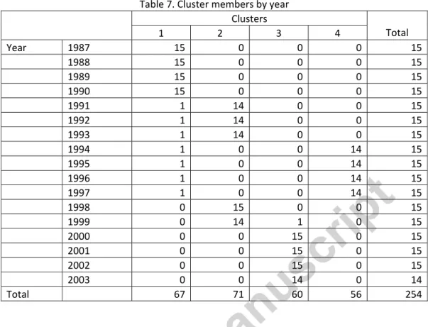
Table 7. Cluster members by year 

  Clusters   

Total 

1  2  3  4 

Year  1987  15 0 0 0  15

  1988  15 0 0 0  15

  1989  15 0 0 0  15

  1990  15 0 0 0  15

  1991  1 14 0 0  15

  1992  1 14 0 0  15

  1993  1 14 0 0  15

  1994  1 0 0 14  15

  1995  1 0 0 14  15

  1996  1 0 0 14  15

  1997  1 0 0 14  15

  1998  0 15 0 0  15

  1999  0 14 1 0  15

  2000  0 0 15 0  15

  2001  0 0 15 0  15

  2002  0 0 15 0  15

  2003  0 0 14 0  14

Total    67 71 60 56  254

The time‐wise structure of clusters shows a picture that is very different from the country‐

wise one. It suggests cycles in the effect of sectoral structure on inventory investment: 1987‐

1990 (four years), 1991‐1993 (three years), 1994‐1997 (four years), 1998‐1999 (two years)  and 2000‐2003 (four years). Cluster 1 is dominated by data from 1987‐1990 (in that cycle,  inventory investments were higher than average and agriculture and manufacturing had  significantly larger than average weight; see Table 7). Table 8 also showed that Cluster 1 was  the most inventory intensive cluster, a fact that fits the sectoral characteristics. In Cluster 2,  there are members from two different shorter time periods (1991‐1993 and 1998‐1999) and  Cluster 4 contains data from 1994‐1997. Cluster members have a below average weight of  manufacturing and agriculture, and these clusters show a smooth transition to Cluster 3 in  terms of sectoral structure. Cluster 3 is dominated by data from 2000‐2003, and both the  manufacturing and agriculture industries have their lowest average share in the sectoral  structure. If we refer to Table 8 again, we can see that Clusters 2 and 3 have below average  inventory intensities, and that between two periods of Cluster 2, Cluster 4 has above  average intensity. The low inventory intensity of Cluster 3 can be easily explained because it  has the lowest shares of agriculture and manufacturing (the most inventory‐intensive  industries) in the sectoral structure. Unfortunately, this phenomenon alone does not explain  the difference between Clusters 2 and 4 because the sectoral structures are very similar on  average in these clusters.  

Summarising our findings, Table 7 shows a trend of movement of the countries from Cluster  1 to Cluster 3 via Clusters 2 and 4. The proportions of agriculture and manufacturing are the  highest in Cluster 1 and are the lowest in Cluster 3; the other two clusters represent  transitional periods. 

4. Sectoral and national inventory investments   

Tables 8 and 9 display sectoral inventory investment data for the six countries. 

Table 8. Average contribution to GVA% 

Sector  Country 

Agriculture  Manufacturing  Construction  Trade 

Austria  2.92  20.23  7.57  13.36 

Finland  4.64  23.60  5.95  10.51 

Ireland  6.84  29.21  6.84  10.27 

Italy  3.21  21.77  5.39  13.55 

The Netherlands  3.47  17.20  5.70  13.22 

United Kingdom  1.52  19.95  5.56  11.45 

Average  3.77  21.99  6.17  12.06 

Table 9. Sectoral inventory intensity (in % of the industrial VA)  Sector 

Country 

Agriculture  Manufacturing  Construction  Trade 

Austria  5.76  .60  .09  1.65 

Finland  ‐1.49  1.06  ‐ .10  ‐ .34 

Ireland  .15  1.74  NA  3.29 

Italy  .97  1.51  NA  NA 

The Netherlands  1.04  .89  .04  .11 

United Kingdom  .42  ‐ .36  .58  1.97 

Average  .22*  .96  .15  1.74 

* without Austria   

The Netherlands is second in the overall (15 countries) ranking of countries in terms of  inventory effectiveness. This position is at least partly a consequence of the fact that out of  the four sectors, only trade’s ratio is higher than average, and this sector has performed  remarkably well. Italy’s position cannot be discerned due to lack of data. The UK has the  third lowest level of long‐term inventory investment. This is closely connected to the unique  feature that the UK has decreased its manufacturing inventories, and manufacturing is  usually the  largest contributor  to  increasing inventory investments.  The  other  three  countries all belong to the high inventory intensity category. In case of Finland, this can be  explained by the high ratio of manufacturing to GVA, especially because it is anecdotally  known that within manufacturing the industries with the highest average inventories are  dominant (electronics and machinery). As was seen in the cluster analysis, Ireland behaves  rather irregularly compared to the other countries, though that countries the relatively high  inventory investments can be attributed to the high proportion of manufacturing (the  highest in the group). This is not compensated by a large weight of agriculture because its  agricultural inventories are relatively low. We could not find any explanation for the high  inventory investments in Austria because, according to detailed data, both the sectoral  structure and the sectoral inventory intensity should have led to a lower long‐term average. 

Conclusion   

The relationship between economic sectors and the ratio of inventory investment per Gross  Value Added in developed countries is not at all straightforward. We made many various  calculations  that exposed some  characteristics of that connection, but a  number of  questions remain unanswered. The hypothesis that there is a relationship between sectoral  structure and inventory intensity can be accepted – it has been proven by our cluster  analysis results and the correlation analysis as well. We can also say that the higher the  proportion of manufacturing and agriculture in the production of GVA, the higher the  inventory intensity of the country. We cannot make similarly definite statements about the  role of construction and trade. Within manufacturing, the chemical, mechanical, metallurgy  and electronics industries are important: their major share leads to a relatively higher  inventory level. The analysis also supports the otherwise trivial conclusion that the main  factor lowering inventories in the long run is the increasing share of services. 

We did not find any significant correlation between annual changes in inventory investments  and sectoral structure. This is not surprising because structural changes have longer‐term  features than the factors that change annual inventories. However, it is shown that, in the  long run, sectoral changes do accompany changes in inventory behaviour. For more  conclusive results, further research, including the examination of national case studies, is  required. 

References   

- Blinder, A.S.‐ Maccini, L. (1991):  The Resurgence of Inventory Research: What Have  We Learned?," Journal of Economic Surveys, Blackwell Publishing, Vol. 5(4), pages  291‐328.  

- Chikán, A. (1981): Market Disequilibrium and the Volume of Stocks. In: Chikan, A (ed,  1981): The Economics and Management of Inventories. Elsevier, Amsterdam  ‐  Akademiai Kiado, Budapest 

- Chikán, A. (1994): Judging Global Inventory Trends −   A Connection of Macro and  Micro Analyses. In: Chikan, A. − Milne, A. −Sprague, L. G. (eds): Reflection on Firm  and National Inventories. International Society for Inventory Research, Budapest. 

- Chikán, A. – Horváth, C. (1999): A multi‐country analysis of aggregate inventory  behavior, International Journal of Production Economics, Vol. 59 (1‐3), pp. 1‐11. 

- Chikán, A. – Kovács, E. (2009): Inventory Investment and GDP Characteristics in  OECD countries, International Journal of Production Economics, Vol. 118 (1), pp. 2‐9. 

- Chikán, A. – Kovács, E. – Tátrai, T. (2005): Macroeconomic characteristics and  inventory investment: a multi‐country study, International Journal of Production  Economics, Vol. 93‐94, pages 61‐73. 

- Chikán, A. – Milne, A. – Sprague, L. G. (eds.) (1994): Reflection on Firm and National  Inventories. International Society for Inventory Research, Budapest. 

- Chikán,  A. – Tátrai, T. (2003): Developments in  global inventory investment,  International Journal of Production Economics, Vol. 81‐82, pp. 13‐26. 

- Dimelis, S. P. (2001): Inventory investment over the business cycle in the EU and the  US, International Journal of Production Economics, Vol. 71 (1‐3), pp. 1‐8. 

- Dimelis, S. P. – Lyriotaki, M. N. (2007): Inventory investment and foreign ownership  in Greek manufacturing firms, International Journal of Production Economics, Vol. 

108 (1‐2), pp. 8‐14. 

- Ehemann, C. (2004): An alternative estimate of real inventory change for national  economic accounts, International Journal of Production Economics, Vol. 93‐94, pp. 

101‐110. 

- Guariglia – Mateut (2010): Inventory investment, global engagement, and financial  constraints in the UK: Evidence from micro data, Journal of Macroeconomics, Vol 32  (1), pp. 239‐250. 

- Hirsch, A. A. (1996): Has inventory management in the US become more efficient  and flexible? A macroeconomic perspective, International Journal of Production  Economics, Vol. 45 (1‐3), pp. 37‐46. 

- Humphreys, B. R. (2001): The behavior of manufacturers’ inventories: Evidence from  US industry level data, International Journal of Production Economics, Vol. 71 (1‐3),  pp. 9‐20. 

- Humphreys, B. R – Maccini, L. J. – Schuh, S. (2001): Input and output inventories,  Journal of Monetary Economics, Vol. 47 (2), pp. 341‐375. 

- Irvine, F. O. (2003a): Long term trends in US inventory to sales ratios, International  Journal of Production Economics, Vol. 81‐82, pp. 27‐39. 

- Irvine, F. O. (2003b): Problems with using traditional aggregate inventory to sales  ratios, International Journal of Production Economics, Vol. 81‐82, pp. 41‐50. 

- Irvine, F. O. (2005): Trend breaks in US inventory to sales ratios, International  Journal of Production Economics, Vol. 93‐94, pp. 13‐23. 

- Irvine,  F.  O.  – Schuh,  S.  (2005):  Inventory investment and  output  volatility,  International Journal of Production Economics, Vol. 93‐94, pp. 75‐86. 

- Kornai, J. (1980): The Economics of Shortage, North‐Holland, Amsterdam 

- Lovell,  M.C. (1994):  Researching Inventories: Why haven’t we  learned more? 

International Journal of Production Economics, Vol. 35 (1‐3), pp. 33‐41. 

- Malgarini, M (2007): Inventories and business cycle volatility: an analysis based on  ISAE survey data, ISAE Working papers No 84 

- Stern, A. (2001): Multiple regimes in the US inventory time‐series: A disaggregate  analysis,  International Journal of Production Economics, Vol. 71 (1‐3), pp. 45‐53. 

‐  West, K. D. (2002): A comparison of the behavior of Japanese and US inventories,  International Journal of Production Economics, Vol. 26 (1‐3), pp. 115‐122. 

- www.oecd.org   

Appendix 1. Contribution of the four main sectors to Gross Value Added and its change (%) 

Agriculture  Manufacturing  Construction  Trade  Services 

Germany  1987‐2003  1.32 24.67 5.69 10.36 48.13 

Change*  0.78 0.76 0.88 1.07 1.19 

Netherlands  1987‐2003  3.47  17.20  5.70  13.22  46.75 

Change*  0.61 1.06 0.71 0.90 1.14 

Canada  1987‐2003  2.69 17.88 5.70 11.34 45.26 

Change*  0.78 1.08 0.78 0.95 1.03 

Italy  1987‐2003  3.21 21.77 5.39 13.55 40.84 

Change*  0.78 1.08 0.78 0.95 1.17 

Japan  1987‐2003  1.86 22.88 8.04 13.63 43.55 

Change*  0.60  0.91  0.93  0.94  1.22 

France  1987‐2003  3.17 18.99 5.81 10.70 50.97 

Change*  0.75 0.86 0.82 0.93 1.13 

Sweden  1987‐2003  2.60 20.93 5.01 10.78 47.59 

Change*  0.78 0.76 0.88 1.07 1.11 

UK  1987‐2003  1.52 19.95 5.56 11.45 45.44 

Change*  0.53 0.72 0.85 1.08 1.20 

Denmark  1987‐2003  3.40 16.67 5.01 12.68 49.29 

Change*  0.60  0.91  0.93  0.94  1.04 

USA  1987‐2003  1.33 16.35 4.22 13.04 52.67 

Change*  0.61 0.84 1.04 0.98 1.08 

Spain  1987‐2003  4.49 19.12 7.97 11.33 38.58 

Change*  0.75 0.86 0.82 0.93 1.12 

Finland  1987‐2003  4.64 23.60 5.95 10.51 41.32 

Change*  0.61 1.06 0.71 0.90 1.09 

Austria  1987‐2003  2.92  20.23  7.57  13.16  40.99 

Change*  0.52 0.94 1.12 0.95 1.11 

Ireland  1987‐2003  6.84 29.21 6.84 10.27 36.46 

Change*  0.60 0.84 0.93 0.93 1.05 

Belgium  1987‐2003  1.75 20.05 5.08 12.20 45.91 

Change*  0.60 0.84 0.93 0.93 1.14 

* Change is the ratio of the averages of the last five (1999‐2003) and first five years (1987‐1991).  

Appendix 2. Contribution of the six manufacturing sub‐sectors to Gross Value Added and  its change (%) 

Food  Chemicals  Metallurgy  Machinery  Electronics  Transport vehicles 

Germany  1987‐2003  2.19 3.90 3.24 3.61 3.71 3.34 

Change*  0.87 0.76 0.75 0.79 0.67 0.89 

Netherlands  1987‐2003  3.18 3.49 1.99 1.29 1.70 0.78 

Change*  0.98 0.75 0.71 0.91 0.69 0.95 

Canada  1987‐2003  2.39 2.61 2.22 1.14 1.24 2.64 

Change*  0.89 0.97 1.03 1.20 0.95 1.48 

Italy  1987‐2003  2.25 3.00 3.02 2.51 2.07 1.33 

Change*  0.87 0.86 0.82 0.88 0.77 0.81 

Japan  1987‐2003  2.55 3.32 2.95 2.25 4.13 2.38 

Change*  0.85 0.95 0.64 0.72 0.83 0.92 

France  1987‐2003  2.69 3.34 2.54 1.50 2.25 2.02 

Change*  0.89 1.01 0.84 0.76 0.82 1.16 

Sweden  1987‐2003  1.82 2.75 2.85 2.66 2.38 2.76 

Change*  0.97 1.25 0.94 1.06 1.04 1.05 

UK  1987‐2003  2.75 3.49 2.24 1.68 2.47 2.04 

Change*  0.73 0.72 0.64 0.69 0.74 0.73 

Denmark  1987‐2003  3.01 2.46 1.73 2.41 1.71 0.61 

Change*  0.80 1.21 0.99 0.90 1.13 0.68 

USA  1987‐2003  1.73 2.76 1.82 1.19 2.25 2.02 

Change*  0.87 0.90 0.78 0.74 0.83 0.80 

Spain  1987‐2003  3.16 3.12 2.32 1.22 1.43 2.06 

Change*  0.69 0.84 0.89 0.91 0.74 0.92 

Finland  1987‐2003  2.27 2.58 2.55 2.74 3.68 1.01 

Change*  0.64 0.99 1.06 0.96 2.87 0.75 

Austria  1987‐2003  2.24 2.35 3.16 2.29 2.53 1.13 

Change*  0.80 0.94 0.91 1.03 0.98 1.46 

Ireland  1987‐2003  6.24 8.68 0.90 1.06 5.91 0.49 

Change*  0.73 2.68 0.59 0.49 1.47 0.68 

Belgium  1987‐2003  2.63 4.75 3.07 1.28 1.65 1.90 

Change*  0.88 1.02 0.68 0.79 0.81 0.77 

* Change is the ratio of the average of the last five (1999‐2003) and first five years (1987‐1991). 

Appendix 3. Average proportion of the contribution of the main sectors to GVA production,  1987‐2003  

  Agriculture  Manufacturing Construction  Trade  Services* 

Germany  1.32  24.67 5.69 10.36 48.13 

Netherlands  3.47  17.20  5.70  13.22  46.75 

Canada  2.69  17.88  5.70  11.34  45.26 

Italy  3.21  21.77  5.39  13.55  40.84 

Japan  1.86  22.88 8.04 13.63 43.55 

France  3.17  18.99  5.81  10.70  50.97 

Sweden  2.60  20.93  5.01  10.78  47.59 

UK  1.52  19.95  5.56  11.45  45.44 

Denmark  3.40  16.67 5.01 12.68 49.29 

USA  1.33  16.35  4.22  13.04  52.67 

Spain  4.49  19.12  7.97  11.33  38.58 

Finland  4.64  23.60 5.95 10.51 41.32 

Austria  2.92  20.23 7.57 13.16 40.99 

Ireland  6.84  29.21  6.84  10.27  36.46 

Belgium  1.75  20.05  5.08  12.20  45.91 

* Finance, insurance, real estate, business, community, social and personal services   

Appendix 4. Change of the proportion of the main sectors in GVA* production   

  Agriculture  Manufacturing  Construction  Trade  Services* 

Germany  0.78  0.76  0.88  1.07  1.19 

Netherlands  0.61  1.06  0.71  0.90  1.14 

Canada  0.78  1.08 0.78 0.95 1.03 

Italy  0.78  1.08  0.78  0.95  1.17 

Japan  0.60  0.91  0.93  0.94  1.22 

France  0.75  0.86 0.82 0.93 1.13 

Sweden  0.78  0.76 0.88 1.07 1.11 

UK  0.53  0.72  0.85  1.08  1.20 

Denmark  0.60  0.91  0.93  0.94  1.04 

USA  0.61  0.84 1.04 0.98 1.08 

Spain  0.75  0.86  0.82  0.93  1.12 

Finland  0.61  1.06  0.71  0.90  1.09 

Austria  0.52  0.94  1.12  0.95  1.11 

Ireland  0.60  0.84 0.93 0.93 1.05 

Belgium  0.60  0.84  0.93  0.93  1.14 

* Ratio of five year average annual proportions between (1999‐2003) and (1987‐1991) 

** Finance, insurance, real estate, business, community, social and personal services