Statistical Phenomena in Astronomy

(1)

Lajos G. Bal´azs

August 11, 2004

(2)

(3)

8 Physical difference between GRBs 109 8.1 Basic characteristics of GRBs . . . 109 8.2 Analysis of the duration distribution . . . 110 8.2.1 Comparison of T90 and T50 statistical properties . . . . 113 8.3 Analysis of the fluence distribution . . . 114 8.4 Correlation between the fluence and duration . . . 117

8.4.1 Effect of the detection threshold on the joint probability distribution of the fluence and duration . . . 118 8.4.2 Intrinsic relationship between the fluence and the du-

ration . . . 119 8.4.3 Maximum Likelihood estimation of the parameters via

EM algorithm . . . 121 8.4.4 Possible sources of the biases . . . 126 8.5 Discussion . . . 132

IV Summary and theses 135

(6)

(7)

Part I

Mathematical introduction

7

(8)

(9)

Chapter 1 Nature of astronomical information

The information we receive from Cosmos is predominantly in the form of electromagnetic radiation. An incoming plain wave can be characterized by the following quantities:

n(direction), λ(wavelength), polarization.

These physical quantities determine basically the possible observational pro- grams:

1. Position =⇒Astrometry

2. Distr. of photons with λ=⇒Spectroscopy 3. Number of photons =⇒ Photometry 4. Polarization =⇒ Polarimetry

5. Time of observation =⇒variability

6. Distr. of photons in Data space =⇒Statistical studies

In the reality, however, not all these quantities can be measured simulta- neously. Restriction is imposed by the existing instrumentation.

By observing and storing the photons of the incoming radiation typically we get a data cube defined by (α, δ, λ). The measuring instrument has some finite resolution in respect to the parameters of the incoming radiation. Con- sequently, the data cube can be divided into cells of size of the resolution.

The astronomical objects can be characterized by isolated domains on the 9

(10)

α, δ plane. A real object can be more extended than one pixel in this plane.

An object is called point source if it occupies an isolated pixel.

Each pixel in the α, δ plane can have a set of non-empty cells according to the different λ values. A list of non-empty pixels can be ordered into a matrix form having columns of properties (α, δ, and the set of λs) and rows referring to the serial number of objects. This structure is the ’Data Matrix’

which is the input of many multivariate statistical procedures.

Table 1.1: Structure of the Data Matrix: m means the number of properties and n runs over the cases.

α₁ δ₁ λ₁₁ λ₁₂ · · · λ_1m α2 δ2 λ21 λ22 · · · λ2m

... ... ... ... ... ...

α_n δ_n λ₁₁ λ₁₂ . . . λ_nm

1.1 Brief summary of multivariate methods

1.1.1 Factor Analysis

A common problem in the multivariate statistics whether the stochastic variables described by different properties are statistically independent or can be described by a less number of physically important quantities behind the data observed. The solution of this problem is the subject of the factor analysis.

Factor analysis assumes a linear relationship between the observed and the background variables. The value (factor scores) and number of background variables, along with the coefficients of the relationship (factor loadings) are outputs of the analysis. The basic model of factor analysis can be written in the following form:

Xj =

Xm k=1

ajkFk+uj , (j = 1,· · ·, p). (1.1) In the formula above X_j mean the observed variables, pthe no. of properties,mthe no. of hidden factors (normally m < p),a_jk the factor loadings, F_k the factor scores, and u_j called individual factors. The individual factors represent that part of the observed variables which are not explained by the common factors.

A common way to solve the factor problem uses the Principal Compo- nents Analysis (PCA). PCA has many similarity with the factor analysis,

(11)

however, its basic idea is different. Factor analysis assumes that behind the observed ones there are hidden variables, less in number, responsible for the correlation between the observed ones. The PCA looks for uncorrelated background variables from which one obtains the observed variables by linear combination. The number of PCs equal to those of the the observed variables. In order to compute the PCs one have to solve the following eigenvalue problem:

R a = λa (1.2)

where R,a and λ mean the correlation matrix of the observed variables, its eigenvector and eigenvalue, respectively. The components of the a eigenvectors gives the coefficients of the linear relationship between the PCs and the observed variables. The PC belonging to the biggest eigenvalue of R gives the most significant contribution to the observed variables. The PCs can be ordered according the size of the eigenvalues. In most cases the de- fault solution of the factor problem is the PCA in the statistical software packages (BMDP, SPSS, ...). Normally, if the observed variables can be described by a less number of background variables (the starting assumption of the factor model) there is a small number of PCs having large eigenvalue and their linear combination reproduce fairly well the observed quantities.

The number of large eigenvalues gives an idea on the number of the hidden factors. Keeping only those PCs having large eigenvalues offers a solution for the factor model. This technique has a very wide application in the different branches of observational sciences. For the astronomical context see Murtagh & Heck (1987).

The factor model can be used successfully for separating cosmic structures physically not related to each other but projected by chance on the same area of the sky. We will return to the details later on when dealing with case studies.

1.1.2 Cluster Analysis

Factor analysis is dealing with relationships between properties when describing the mutual correlations of observed quantities by hidden background variables. One may ask, however, for the relationship between cases. In order to study the relationship between cases one have to introduce some measure of similarity. Two cases are similar if their properties, the value of their observed quantities, are close to each other.

”Similarity”, or alternatively ”distance” between l andk cases, is a function of twoX_j^l,X_j^k set of observed quantities (j is running over the properties

(12)

describing a given case). Conventionally, if l = k, i. e. the two cases are identical, the similarity a(X_j^l, X_j^k) = 1 and the distanced(X_j^l, X_j^k) = 0. The mutual similarities or distances of cases form a similarity or distance matrix.

Forming groups from cases having similar properties according to the measures of similarities and the distances is the task of cluster analysis.

There are several methods for searching clusters in multivariate data. There is no room here to enter into the details. For the astronomical context see again (Murtagh & Heck , 1987). Typical application of this procedure is the recognition of celestial areas with similar properties, based on multicolor observations. The procedure of clustering in this case is a searching for pixels on the images taken in different wavelengths but having similar intensities in the given colors.

In the following we try to demonstrate how these procedures are working in real cases.

(13)

Chapter 2 The basic equation of stellar statistics

2.1 Formulation of the problem

It is a basic problem in astronomy that we can not measure quantities di- rectly, e.g. linear extension, space velocity or absolute brightness. Instead, we can get only their distance-dependent apparent values (angular diameter, proper motion, apparent brightness). In general, there exists a relationship in the form of

e=e(E, r) , (2.1)

wheree,E andrare the measured value, the true value, and the distance, respectively. Following the law of full probabilities we may write:

φ(e) =

Z

φ(e|r)g(r)dr . (2.2)

In this expression φ(e), φ(e|r) and g(r) are the probability density of e, the conditional probability of e, given r, and the probability density of r, respectively. Since the measured distance-dependent values can be written in the forme=Eβ(r) in the cases we consider, whereβ(r) =r⁻ⁿif we neglected interstellar absorption and cosmological effects, one can reduce e = e(r, E) to z =x+y with a suitable logarithmic transformation. (n = 1 for angular diameters and proper motions while n= 2 for apparent brightness).

Supposing the statistical independence of yand z we get the convolution equation between the probability densities of these variables:

h(z) =

Z

f(z−y)g(y)dz . (2.3)

13

(14)

This equation is also called the basic equation of stellar statistics.

2.2 Solutions of the basic equation

The task is to findg(y) ifh(z) and f(x) are given. The convolution equation is a Fredholm type integral equation. Its formal solution can be obtained by Fourier transformation. This solution has little practical use because we generally know only a statistical sample drawn from h(z). There are several methods for obtaining the moments ofg(y), its approximation in form of orthogonal series, or its numerical values at discrete points. Particular attention will be devoted to computing the maximum likelihood estimate of the discrete values of g(y) via the EM algorithm.

2.2.1 Eddington’s solution

Let us assume thatf(x) and g(y) are the probability densities of the statis- tically independent random variables xand y.

By definition z =x+y, and the probability density h(z) of the observed quantity z is connected withf(x) and g(y) by the convolution equation.

Suppose thath(z) has derivativesh^(k)(z) of all orders andf(x) has central moments, µ_k. We look for the solution of the convolution equation in the form of a series, g(z) = ^P^∞

0 γ_kh^(k)(z). (Eddington 1913; uniqueness of the solution and convergence of the series are discussed by Kurth 1952).

Writing

h(z) =

+∞Z

−∞

f(x)g(z−x)dx (2.4)

and expanding g in a Taylor series around z we obtain h(z) =

+∞Z

−∞

f(x)

X∞ k=0

(−x)^k

k! g^(k)(z)dx. (2.5)

Integrating term by term and supposingEx= 0 (E here meaning expectation value) we get

h(z) =

X∞ k=0

g^(k)(z)(−1)^k

k! µ_n. (2.6)

Now we substitute the formal series

(15)

h(z) =

X∞ k=0

X∞ m=0

γ_mh^(k+m)(z)(−1)^k

k! µ_k. (2.7)

Introducing n =k+m, the double sum can be written in the form h(z) =

X∞ n=0

h⁽ⁿ⁾

Xn k=0

γ_n−k(−1)^k

k! µ_k. (2.8)

The equation is satisfied if on the right side the coefficients of h⁽ⁿ⁾except n= 0 equal zero. This means

γ₀ = 1

Xn k=0

γ_n−k(−1)^k

k! µ_k = 0, n6= 0. (2.9) Based on these equalities the coefficients γ_k of the formal series can be expressed by the central moments µ_k of f

γ₀ = 1 ,

γ₁ = 0,

γ2 =−¹₂µ2 =−¹₂σ², γ₃ = ¹₆µ₃,

γ₄ =−₂₄¹µ₄+¹₄µ²₂, etc. (2.10) For small values of µ₂ = σ² the above equalities suggest approximating the solution g(y) by the function

h(y)− 1

2σ²h⁰⁰(y). (2.11)

In real cases, however, it is rather inconvenient to compute the second derivativeh⁰⁰(y) numerically. One may therefore replace it by the ratio

α⁻²[h(y+α) +h(y−α)−2h(y)], (2.12) where α is a small positive number. As shown by the Taylor theorem, the difference between h⁰⁰ and the above formula is of the fourth order in α. Using this expression for the second derivative one obtain the following approximation

g₂(y) = h(y)− 1 2(σ

α)²[h(y+α) +h(y−α)−2h(y)]. (2.13)

(16)

In an analogous way one can derive a ”five-point formula”, a ”seven point formula” etc. in order to get the higher order derivatives. In applications, however, derivatives of order higher than 4 are not used because of the increasing uncertainty of the estimation of moments with increasing order.

2.2.2 Solution by Fourier transformation

A formally simple method of analytic solution of the basic equation is the Fourier transform one. Taking the Fourier transform of both sides of the equation yields

ˆh(ν) =√

2π f(ν) ˆˆ g(ν) (2.14) where ν is the frequency. It is easy to get from this equation an analytic solution

g(y) = 1 2π

+∞Z

−∞

ˆh(ν)

f(ν)ˆ e^iνydν. (2.15)

In real cases, however, h(z) is known only in terms of a sample drawn from it and one may approximate the original probability density function with an arbitrarily small error as the sample sizen goes to infinity. A given sample size sets a bound within which the different solutions of the basic equation are statistically indistinguishable.

Suppose we have a solution obtained by applying the above formula. One may add to ˆg(ν) aδ(ν) function in the frequency domain which has a constant value in a {ν₀, ν₀+ ∆ν} region and 0 otherwise. Since the existence of the Fourier transformation requires ^R fˆ(ν)²dν < ∞ , √

2π fˆ(ν) [ˆg(ν) + δ(ν)]

approaches arbitrarily closely to ˆh(ν), and after Fourier transformation h(z), asν₀ goes to infinity.

The Fourier counterpart of δ(ν) is a high frequency oscillating function which one may add to the g(y) solution without violating the statistical bound around h(z), i.e. ^R[ˆg(ν) +δ(ν)]exp(iνx)dx may also be accepted as a solution. Increasing the sample size n decreases the statistical bound as

√n. Hal´asz (1984) showed, however, that the bound around theg(y) solution decreases only as log(n) at the same time.

An obvious way out of this difficulty appears to be to apply some cut-off frequencyν₀, i.e to integrate in the {−ν₀;ν₀}domain instead of{−∞; +∞}.

Proceeding in this way, however, one has some problem in selecting the ’best value’ for ν₀ which makes this procedure somewhat arbitrary.

Another, at first glance appealing, approach appears to be developing the h(z) probability density into an orthogonal series:

(17)

h(z) =

X∞ k=0

akHk(z)α(z), where ak = 1 k!

+∞Z

−∞

Hk(z)h(z)dz. (2.16) Here the α(z) = exp(−z²/2)/√

2π and Hk(z) are Hermite polynomials.

Applying the Fourier transformation to the Hermite functions H_k(z)α(z) we obtain

Hˆ_k(ν) =√

2π(iν)^kα(ν). (2.17)

(For further details see Kendall & Stuart, 1973, Vol1, pp. 156-157). The solution of the basic equation by the Fourier method reduces then to solving the equations

α(z)Hk(z) =

+∞Z

−∞

f(z−y)gk(y)dx, gk(y) = 1

√2π

+∞Z

−∞

(iν)^kα(ν)

fˆ(ν) e^iνydν. (2.18) If these integrals exist, we get the solution in form of g(y) = ^P^∞

k=0a_kg_k(y).

This approach seems to overcome the difficulty of high frequency noise occurring in the solution. Computing the higher ordera_k coefficients, however, one get increasing uncertainty due to the sampling error of h(z).

2.2.3 Malmquist’s solution

In deriving the basic equation we used the law of full probability. Formally, based on this theorem, we may write the g(y) solution as

g(y) =

Z

g(y|z)h(z)dz (2.19)

where g(y|z) is the conditional probability assuming z, the measured quantity, is given. If one succeeds in developing g(y|z), the solution is given by computing the integral given above.

In some important cases, as Malmquist (1924, 1936) recognized, the momenta can be developed without knowing g(y|z) itself. Let z be a unit random variable and h(z) its probability density. It may be represented as

√1

2πe⁻¹²^z²[1 +γ3H3(z) +γ4H4(z) +...], (2.20) where

(18)

γ₃ = ^√¹_3!µ₃,

γ4 = ^√¹_4!(µ4−3) (2.21)

and µ₃, µ₄ are the central moments of z of the third and fourth order.

Hk(z)−s are the orthogonal functions of the ”Hermite’s polynomials” and the series obtained is called the ”Gram-Charlier series” (cf. Kendall & Stuart, 1973, Vol 1, pp 156-157). If z is not a unit variate the corresponding series can be obtained using the unit variate ζ = (z −µ)/σ by the appropriate transformation. Computing the corresponding moments of the conditional probability we may develop its Gram-Charlier series and, consequently, the g(y) solution.

According to Bayes theorem

g(y|z) = χ(y, z)

R χ(y, z)dy = χ(y, z)

h(z) . (2.22)

Following the notations of the first paragraph we may write χ(y, z) = f(z−y)g(y) and g(y|z) = f(z−y)g(y)

h(z) . (2.23)

In a number of practically important cases f(x) is a gaussian function, i.e. f(x) = exp(−(x− µ)²/2σ²₀)/√

2πσ₀. In this case one need not know g(y) when computing the momenta of the conditional probabilityg(y|z). By definition

µ(z) =

Z

yg(y|z)dz =

R ye

−(z−y−µ)2 2σ2

0 g(y)dy

R e

−(z−y−µ)2 2σ2

0 g(y)dy

. (2.24)

Differentiation of log(h(z)) yields d

dz log(h(z)) =

R _{−(z−y−µ)}

σ²₀ e

−(z−y−µ)2 2σ2

0 g(y)dy

R e

−(z−y−µ)2 2σ2

0 g(y)dy

(2.25) and we get

µ(z) = z−µ+σ₀² d

dz log(h(z)). (2.26)

Similar computation gives an expression for the σ(z) standard deviation of g(y|z)

(19)

σ(z)² =σ₀²[1 + σ²₀ 2

d²

dz² log(h(z))]. (2.27) Higher order moments can be obtained in an analogous way. Substituting these moments into the expression of the Gram-Charlier series we get finally g(y|z) and thusg(y), after performing the integration.

The expressions for the moments of the g(y|z) conditional probability have important consequences, often overlooked in practical applications. Ifz is given by the observations, then the expected value ofy is not simplyz−µ, whereµis the expected value ofx, but has to be corrected by the third term in the expression for µ(z). This term is called the Malmquist correction.

If one determined spectroscopically the absolute magnitude M₀ of a star of apparent magnitude m the expected value of the distance modulus is not simply m−M₀ but a value corrected with the Malmquist’s term.(For more details see Mihalas and Binney (1981)).

2.2.4 Lucy’s algorithm

Lucy (1974) proposed an algorithm for solving the integral equation connecting g(y), g(y|z) and h(z), in an iterative way. Let us assume that at some stage of the iteration we getg^(r)(y), g^(r)(y|z). The estimate (r+ 1) is

g^(r+1)(y) =

Z

g^(r)(y|z)h(z)dz, . (2.28) where, applying Bayes theorem of conditional probabilities,

g^(r)(y|z) = g^(r)(y)h(z|y)

h^(r)(z) . (2.29)

with

h^(r)(z) =

Z

h(z|y)g^(r)(y)dy. (2.30) In the above equalities h(z|y) denotes the conditional probability of z, assumingyis given. In the case whenyandz−yare statistically independent h(z|y) = f(z − y). Since g(y) is a probability density it should fulfil the following relations:

Z

g(y)dy = 1 and g(y)≥0. (2.31) One may readily show that this iterative procedure conserves these con- straints. Eliminating h(z|y) from the above equations we obtain

(20)

g^(r+1)(y) =g^(r)(y)

Z h(z)

h^(r)(z)h(z|y)dy (2.32) from which one can easily recognize that g^(r+1) ≥ 0 if g⁽⁰⁾ ≥ 0. Proof of the conservation of the normalization constraint is straightforward by integration ofg^(r+1)(y) and using the normalizations of the g^(r)(y|z) and h(z) probabilities.

Actually, we know h(z) only in terms of a sample drawn from it and we might be concerned at the loss of information involved in forming a histogram from the data in order to get an ˜h(z) estimate for h(z). The sample itself can be represented by the expression

˜h(z) = 1 N

XN n=1

δ(z−z_n), (2.33)

whereN,z_nand δ(z−z_n) are the size of the sample, the individual measures and Dirac’s delta function, respectively. Substituting this expression into the iterative scheme yields

g^(r+1)(y) = 1 N

XN n=1

g^(r)(y|z). (2.34)

In practice the computation of g(y) is performed on a set of values y_m and the iterative scheme can be interpreted as a procedure for estimating the unknown parameters g_m = g(y_m). In this view the integral expression for h^(r) will be approximated by the following sum

h^(r)(z) =

Xm j=1

g_j^(r)h(z|y_j)∆y. (2.35) The expression obtained in this way allows us to make a comparison with the maximum likelihood (ML) estimation of unknown parameters. If we have a sample of measures z_n then the likelihood function can be written in the form

L(g_j) =

Xn i=1

log(h(z_i)). (2.36)

ML means to maximize L(g_j) over the given sample subject to the constraint ^Pg_j = 1. Applying a λ Lagrange multiplier one has to maximize the following function

G(gj;λ) =L(gj) +λ(

Xm j=1

gj −1). (2.37)

(21)

One finds that the multiplierλ =−n. Performing the differentiation one gets equations for g_j-s maximizingL(g_j)

0 =

Xn i=1

h(z_i|y_j)

Pm

j=1gjh(zi|yj)

−n j = 1, ..., m (2.38)

and multiplication with gj yields gj = 1

n

Xn i=1

gjh(zi|yj)

Pm

j=1g_jh(z_i|y_j) (2.39) which is identical with the last expression of the iteration scheme when it converges (g_j = g_j^(r+1) = g^(r)_j ). Lucy showed that his iteration algorithm monotonically increases the likelihood and converges to the ML solution.

Numerical experiments showed, however, that the ML solution did not give the best fit tog(y) while approximating ˜h(z). This result also presents some hint for the inherent uncertainties of the solution procedures of the basic equation.

2.2.5 The EM algorithm

We have mentioned already in previous sections that in a number of practical cases h(z) is not given analytically but only in a form of a sample drawn from it. To get the solution, therefore, is rather a statistical estimation problem than an analytical procedure for solving integral equations. The true nature of the problem is nonparametric. When one approximates the integral h(z) = ^R h(z|y)g(y)dy by the sum ^P^m

j=1h(z|y_j)g(y_j)∆y, containing g(y_j) (and maybey_j) as unknown parameters, (∆ycan be absorbed intog_j) the solution of the basic equation will be reduced to a parameter estimation problem. The number of parameters, however, is fully arbitrary. Nevertheless, there is a minimum number of parameters still giving a solution within the statistical bound of the sample of h(z).

Replacing the integral with a sum means a discretization of the y statistical variable into y_j, j = 1, ..., m, values. The y_j variable takes these values with g(y_j) =g_j probabilities. We assume furthermore there exists an unobserved vector u = (u₁, ..., u_m) whose components are all zero except for one (the j-th) equal to unity indicating the unobserved y_j state associated with the actually observed z. In the case when both the u and z variables were observed the data would be complete. Their joint probability density would be

(22)

p(z,u) =e

Pm j=1

uj[log(gj)+log(h(z|yj)]

. (2.40)

Since the elements of the vector are zero except a certain u_j, which is unity, p(z, u) reduces to gjh(z|yj) if j is given. To perform a ML estimation we define the likelihood function in the usual form

L(g₁, ..., j_m) = ^Pⁿ

i=1log(p(z_i,u⁽ⁱ⁾)) =

= ^Pⁿ

i=1

Pm

j=1u⁽ⁱ⁾_j [log(g_j) + log(h(z_i|y_j))]. (2.41) Maximizing the likelihood with respect to the gj-s one should take into account the constraint^Pg_j = 1 with a Lagrange multiplierλ. Differentiation with respect to the parametersg_j yields

0 =

Xn i=1

u⁽ⁱ⁾_j gj

+λ= n_j gj

+λ, j = 1, ..., m (2.42)

where n_j is the frequency of occurrence of the j-th state in the sample.

Summing the equations gives λ=−n and substituting it into the equations we get g_j =n_j/n as a ML estimation.

In the case of incomplete data one does not have observations of the states j. Dempster et al. (1977) showed, however, that a ML estimation is still possible if instead ofu we use its conditional expectation assuming that z is given. Proceeding in this way one may estimate g_j-s and the solution is also the ML solution of the case with complete data specification. By definition the conditional probability ofu is given by

v(u|z) = p(z,u)

h(z) and E(u_j|z) =

Z

u_jp(z,u)

h(z) du_j. (2.43) Since u_j has only two values, 0 or 1, the integral is simplified to the form

E(u_j|z) = p(z,u)

h(z) = g_jh(z|y_j)

Pm

j=1g_jh(z|y_j). (2.44) Considering these conditional expected values of theu_j-s as complete data we get the ML estimation in the form

g_j = 1 n

Xn i=1

E(u_j|z) = 1 n

Xn i=1

g_jh(z|y_j)

Pm

j=1g_jh(z|y_j). (2.45)

(23)

Suppose we have an estimateg^(r)_j ofg_j; the next approximationg_j^(r+1)can be obtained if we substituteg_j^(r)into the right side andg_j^(r+1)into the left side.

In this way we recovered Lucy’s algorithm, which is a special case of the EM algorithm, a more general framework for performing ML estimation in cases of incomplete data specification. The convergence and general properties of this algorithm are given by Dempster et al. (1977).

The EM algorithm consists of two steps:

E step: One replaces the unobserved part of the data with the expected values based on their conditional probabilities assuming that the observed part is given.

M step: Using the complete data specification obtained in this way one gets the corresponding ML estimation.

Dempster et al. (1977) showed that performing the E and M steps se- quentially the procedure monotonically converges to the ML solution.

Up to this point they_j parameters have not been included in the parameters to be estimated. The general framework of the EM algorithm, however, allows this generalization without any difficulty. We show this only in a special case when h(z|y_j) = exp(−(z −y_j)²/2σ²_j)/√

2πσ_j. In the case of a gaussian distribution the ML estimation of the y_j and σ_j parameters is the arithmetic mean of z and (z −y_j)². When we are dealing with incomplete data these relations correspond to

y_j =

Pn

i=1ziE(uj|z)

Pn

i=1E(u_j|z) (2.46)

and

σ²_j =

Pn

i=1(z_i−y_j)²E(u_j|z)

Pn

i=1E(uj|z)

. (2.47)

Ifσis independent ofj then we may add a third equation to the equations for y_j and σ_j

σ² =

Xm j=1

g_jσ²_j. (2.48)

These equations could be added to the M step. The estimation of the parameterσ_j is much more uncertain than ofy_j in particular at small sample sizes.

(24)

2.2.6 Dolan’s matrix method

When the integral in the basic equation is approximated by a sum an obvious idea is to solve the resulting system ofn linear equations with respect to the unknowns g(y_j), setting n=m

Xm j=1

f(z_i −y_j)g(y_j)∆y= ˜h(z_i), i= 1, ..., n. (2.49)

˜h(z_i) is obtained from the observed sample of h(z).

This method is rather popular among astronomers due to its simplicity and flexibility since we do not have any particular basis for assumptions about the functions f, g, h. (For further details see Bok (1937)). There are, however, serious problems in practical applications. Unless the sample size is large, the solution of this system of linear equations often yields negative g(y_j)-s violating theg(y_j)≥0 property of probability densities (cf. Trumpler and Weaver 1953, p. 112-114).

The equations can be written in the more compact matrix formFG=H whereF,G,Hare n×n, n×1 andn×1 matrices, respectively. The solution is simply given by G=F⁻¹H requiring the inversion ofF. The large errors occurring in the solution G can be understand if we recognized that application of F on G means some kind of ”smoothing”. The application of the inverse transformation onHamplifies the stochastic fluctuations inherent in obtaining H.

The solution of the system of linear equations requires the inversion of the Fmatrix. Unfortunately, in a number of cases some of the eigenvalues of F are small making the numerical inversion very unstable. To avoid the problem of matrix inversion Dolan (1974) proposed the technique of apodisation (see e.g., Lloyd, 1969). Apodisation constructs the G matrix from the observed H using the known properties of the gaussian ”smoothing” function. A discussion of the numerical accuracy of this procedure is given by Dolan (1972). As shown by Lloyd, the matrix G has elements

g_j =h_j −K{1

2[h_j+l+h_j−l]−h_j} (2.50) wherelis the ”apodisation length” and K is an ”instrument factor” whose value depends on the shape of the smoothing function. For a gaussian function K = (2/π)(σ/l)². The apodisation length, l, should thus be chosen to the nearest integer number to the dispersionσ . The expression given above strongly resembles that obtained in the first approximation of Eddington’s solution.

(25)

2.3 Concluding remarks

All the methods discussed in the present chapter represent different approaches to the same problem. As we mentioned in the introduction there is a typical situation in statistical astronomy where the probability densities of the distance-dependent measurable quantities, of its true physical coun- terparts, and of some distance measures are connected by the convolution equation.

To get the probability density function of the unobserved background variables (e.g. the distance), however, is not a simple analytical procedure of solving a Fredholm-type integral equation of the first kind. Namely, the probability density function h(z) of the observed variable z is not given but has to be estimated somehow from a sample obtained from the observations.

From the analytic properties of the Fredholm integral equations of the first kind it follows that a small deviation fromh(z) is amplified by the solution process in obtaining g(y). This uncertainty is inherent in the equation and can not be overcome by a suitable choice of procedure. In this view the result of Hal´asz (1984) is very significant, i.e. the improvement of the statistical accuracy in gettingh(z) by increase of the sample sizenmeans an improvement in g(y) proportional only to log(n).

Solution procedures may differ in some practical aspects: how they approximate the integral in the equation or the numerical derivatives of h(z) (e.g. in the case of the Eddington or Malmquist methods). These practical aspects could cause particular uncertainties not inherent in other procedures.

The approximation of the integral with a finite sum reduces the solution to the problem of the estimation of unknown parameters behind an observed sample. However, the parameters to be estimated are not in the true sense the values of the unknown g(y) function but its integral over ∆y. Consequently, the accuracy of the estimated parameters follows the general √

n rule of parameter estimation, when n→+∞.

The EM algorithm and its particular case the Lucy algorithm have the nice property of retaining g(y)≥0 for the probability density function of y.

Analytic solutions often suffer from violating this basic property, in particular when the sample size is not large.

The computational efforts are very different among the procedures discussed in this chapter. Obviously, the first approximation of the Eddington solution and the formula given by Dolan are the simplest also from that point of view. The EM algorithm on the other hand requires much more computing time and memory, in particular when the sample size is large, but it has the clear benefit of a sound theoretical basis in mathematical statistics.

This discussion does not attempt to give strict advice on performing so-

(26)

lutions in particular cases. Our aim was rather to call attention to important aspects when trying to find the solution. Our feeling is, however, that the true essence of the problem is more stochastic than analytic and those procedures are superior which retain this basic characteristic.

(27)

Part II

Statistical study of extended sources

27

(28)

(29)

Chapter 3 Separation of Components

3.1 Separation of the Zodiacal and Galactic Light

The IRAS space mission covered the whole sky in four (12, 25, 60, 100 µm) wavelengths. In particular, the 12 and 25 µm images were dominated by the thermal emission of the Zodiacal Light (ZL) having a characteristic temperature around 250K. The contamination of the Galactic Dust thermic radiation by the ZL is quite serious close to the Ecliptic. Assuming that both radiation are coming from optically thin media the observed infrared intensities are sums of those coming from these two components. We may assume furthermore the distribution of the intensity of thermal radiation on the sky coming from the Galactic component has some similarities when observed at the given wavelengths and the same holds also for the ZL. Iden- tifying the radiation coming from these two physically distinct components with the hidden variables in Eq. (1.1) and the incoming intensity with the observed ones the separation of the ZL and the Galactic radiation can be translated into the general framework of factor analysis.

In the case of the IRAS images theRcorrelation matrix has a size of 4×4 by cross correlating the four (12, 25, 60 and 100 µm) images. We selected a field of 15^◦×15^◦ (corresponding to 500×500 pixels) in the Perseus close to the ecliptic and containing the California Nebula, IC 348 and the Pleiades.

Solving Eq. (1.2) in this case we got the results summarized in Tab. 3.1.

One can infer from this table that there are two large eigen values indicating the presence of two important factors. The last two columns of the table give the a_jk factor coefficients for Eq. (1.1). The first factor dominates the radiation at 12 and 25 µm while the second one does it at 60 and 100 µm.

Computing the factor values from the observed data (the measured 12, 25, 29

(30)

Figure 3.1: Input IRAS (12, 25, 60, and 100µm) images of the factor analysis and the resulted two factor pictures. The coordinates are measured in pixels.

The objects are the California Nebula, IC 348 and the Pleiades, in descending order. Note the strong trend in F1 representing the ZL while F2 displays the Galactic component (Bal´azs & T´oth , 1991).

(31)

Table 3.1: Results of factor analysis. There are two large eigen values indicating the presence of two important factors. The last two columns of the table give theajk factor coefficients for Eq. (1.1). (Bal´azs et al. , 1990)

eigen value cum. percent. Variable 1. factor 2. factor

2.4818 62.0 F12 0.9637 0.2089

1.3910 96.8 F₂₅ 0.9917 0.0458

0.1003 99.3 F₆₀ 0.3625 0.9044

0.0268 100.0 F100 0.0409 0.9819

60 and 100 µm intensities) one gets the two images as shown in Fig. 3.1, along with the originals (Bal´azs & T´oth , 1991).

In order to define regions of similar physical properties we performed cluster analysis in the{F₁;F₂} factor plane. These two factors define a two- dimensional subspace in the four-dimensional color space. The 1-st factor almost fully explains the 25 µm flux, which is heavily dominated by the Zodiacal Light and therefore represents its influence in different colors. The second factor, in contrast, describes the effect of the radiation coming from the galactic dust which produces most of the 100 µm emission. Performing cluster analysis altogether 10 regions were defined, however this figure was arbitrary. The result is given in Fig. 3.2. The basic features of this plot are the two ’fingers’ pointing upwards and nearly horizontally. These ’fingers’

may be identified with the Zodiacal Light (dominating F_l) and the galactic radiation (dominating F₂).

The dust emission is basically thermal. We computed the total infrared emission by adding the fluxes in the four bands:

F =F12+F25+F60+F100 (3.1) Assuming a dust emission law in the form of B(T)/λ^α where B(T) is the black body (BB) radiation at T temperature, λ the wavelength and α depend on the physical properties of the emitting dust, we put α = 1.

However, recent studies of the far infrared radiation of the ZL with the ISO satellite indicate nearly BB radiation (Leinert et al. , 2002), i.e α= 0. The specification of α influences the numerical results obtained, of course, but our goal is only to demonstrate the link between the statistical procedure and the physical quantities.

TheF_i/F ratios (iis 12, 25, 60 or 100) depend only onT if a region determined by one characteristic temperature. Supposing the validity of the dust emission law given above we computed the loci of such regions in Fig. 3.2,

(32)

Figure 3.2: Character plot of regions (clusters) of similar properties in the {F₁;F₂} factor plane (left panel). The identical symbols mean physically similar regions. The basic features of this plot are the two ’fingers’ pointing upwards and nearly horizontally. These ’fingers’ may be identified with the Zodiacal Light (dominatingF actor l) and the galactic radiation (dominating F actor2) (Bal´azs et al. , 1990). Distribution of duster members in the {F25/F;F6O/F} plane (right panel). The coding of dusters is the same as in the left panel. The loci of dust low α = 1 radiations of different temperatures are marked with crosses. The numbers in parentheses are the respective temperatures. Note that the wedge-shaped distribution of symbols representing real measurements points towards about 40 K and 200 K dust temperatures (Bal´azs et al. , 1990).

marked with crosses the sources of different temperatures in the line of sight.

As a consequence, the real points in Fig. 3.2 are not on the theoretically computed line but deviate from it according to the relative intensity of superimposed sources of different temperatures. One gets a wedge-shaped distribution of symbols representing real measurements pointing towards about 40K and 200K dust temperatures. This distribution can be obtained from the superimposed ZL and Galactic sources with these characteristic temperatures.

(33)

3.2 Sturucture and Dynamics of the Cepheus Bubble

3.2.1 Basic characteristics

Analysing the IRAS 60µm and 100µm maps of Cepheus, Kun, Balázs and Tóth (1987, hereafter KBT) reported that the area l = 90ô to 106ô, b = +3ô to +10ô is faint at far-infrared wavelengths, and is encircled by a ring- shaped region of enhanced infrared emission, the ‘Cepheus Bubble’. They compared the IRAS maps with Dubout-Crillon’s (1976) Hα photographs, and demonstrated that the brightest parts of the infrared ring correspond to the HII regions IC 1396, Sh2-129, Sh2-133, Sh2-134, and Sh2-140 as well as to fainter or smaller HII regions not listed in Sharpless’ (1959) catalogue.

Since most of the listed brightHII regions were placed at about 900 pc from the Sun in the literature, KBT accepted this value for the Cepheus Bubble as well.

The infrared ring is probably related to the 6ô loop structure discovered atl = 103ô, b= +4ô by Brand and Zealey (1975) as semi-circular filamentary dust lanes and faint emission nebulosity on the POSS prints. They associate this structure with Cep OB2 by noting that to the west the dust seems to interact with IC1396, although in their Table 1 erroneously Cepheus OB1 is given as related OB association. In the area encircled by the infrared ring a deficiency inHIcolumn density was observed by Simonson and van Someren Greve (1976, hereafter SVSG) in the [−20,−6] kms⁻¹ radial velocity range.

The infrared ring coincides positionally with the OB association Cepheus OB2, which consists of two subgroups: the older and more dispersed one, Cep OB2a ( t ≥ 8 × 10⁶yrs, de Zeeuw and Brand (1985)) occupies the interior of the ring, while the younger and smaller subgroup, Cep OB2b (t= 4×10⁶yrs, SVSG) is situated at the edge of the ring. Since the distance of Cepheus OB2 is also about 900 pc, KBT proposed a physical link between the association and the bubble. A similar link was assumed earlier by SVSG, interpreting the low HI content in the region as a sign of the full ionization of the interstellar gas by the Cep OB2 association.

KBT proposed that the Cepheus Bubble had been created by the strong stellar wind/UV radiation and the subsequent supernova explosion of the most massive star in the older subgroup Cep OB2a. The exploded star was perhaps the former companion of the runaway star λ Cep whose proper motion points backwards approximately to the centre of the bubble. From tracing back this motion, KBT estimated an age of 3×10⁶yrsfor the bubble.

The proper motion measured by the Hipparcos satellite does not significantly

(34)

change this age estimate. The formation of the younger subgroup, Cep OB2b could have been triggered by stars of Cep OB2a via stellar wind and propa- gating ionization fronts as proposed by KBT and Patel et al. (1995). This trigger could also be responsible for the birth of OB stars and cold embedded IRAS sources along the periphery of the Cepheus Bubble (KBT, Bal´azs &

Kun, 1989).

De Zeeuw et al. (1999) determined the distances of nearby OB associ- ations using proper motions and parallaxes measured by Hipparcos. Their work on 49 members of Cep OB2 resulted in a distance of 559±30pc, significantly lower than the 900pcassumed before. However, the recalibration of the upper main sequence, suggested by Hipparcos, would also lessen the distance of those objects along the periphery of the bubble (HII regions and reflection nebulae) which were used as distance indicators for the Cepheus Bubble by KBT. Thus the arguments for the physical connection of the bubble with Cep OB2 are probably not affected by the new distance values. Therefore further investigations are needed before accepting the shorter Hipparcos scale.

A better understanding of the history of this Cepheus region requires more detailed mapping of the interstellar matter (including better distance estimates) as well as information on the large scale motions. Velocity information can also help to separate distinct interstellar features projected on the IRAS images. Recently, Patel et al. (1998) conducted a CO(1−0) spectral line survey in Cepheus and discussed the origin and evolution of the Cepheus Bubble on the basis of the overall distribution of molecular gas.

They also performed an HI survey and concluded that the bulk of the interstellar gas associated with the bubble is in atomic form. In this section we investigate the large scale morphology and kinematics of the Cepheus Bubble by a detailed analysis of the distribution of atomic hydrogen.

In the following we analyse HI 21 cm measurements taken from the Leiden/Dwingeloo survey, in order to identify the atomic gas component of the Cepheus Bubble. In addition to the more traditional methods, the analysis of the HI maps is also performed by using multivariate statistical methods. After connecting these new pieces of information into a coherent picture, we speculate about the possible origin of the Cepheus Bubble.

3.2.2 Distribution of neutral Hydrogen

TheHIdata were taken from the Leiden/DwingelooHIsurvey (Hartmann &

Burton, 1997). The angular and velocity resolution of the spectra are 36’ and 1.03kms⁻¹, respectively, covering the velocity range [−450,+450]kms⁻¹. The observed positions are distributed on a regular grid with steps of 0.5^o both in l and b. This grid provides a spatial resolution of up to 3 times

(35)

higher than obtained by SVSG, although the Leiden/Dwingeloo sampling is somewhat coarser than that of the HI data set of Patel et al. (1998).

HI distribution in the channel maps In the region l = 95ô to 110ô, b= 0ô to +15ô HI emission is dominated by a narrow galactic plane layer of b <+6ô at any radial velocity between−110kms⁻¹ and 20kms⁻¹. Although HI emission is detectable over a large range in both b and V_LSR, atb >+6ô the most prominent emission features appear in two discrete velocity intervals at [−155,−135]kms⁻¹ and [−45,+20]kms⁻¹. The HI structure at V_LSR '

−145kms⁻¹ belongs to the extended Outer Arm high velocity cloud (Wakker and van Woerden, 1991), whose study is beyond the scope of this work.

We focus on the [−45,+20]kms⁻¹velocity range, and search for hydrogen structures possibly associated with the infrared ring found in the IRAS maps.

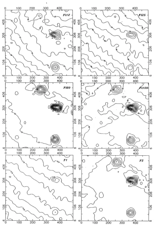
We display in Fig. 3.3 and 3.4 a series ofHI maps by integrating the spectra over 4kms⁻¹ velocity intervals between −38kms⁻¹ and +10kms⁻¹. The maps show that the bulk of HI emission arises from the [−14,+2]kms⁻¹ velocity range. Since the infrared ring is expected to correlate with the projection of the most prominentHI features on the sky, we plotted in Fig.

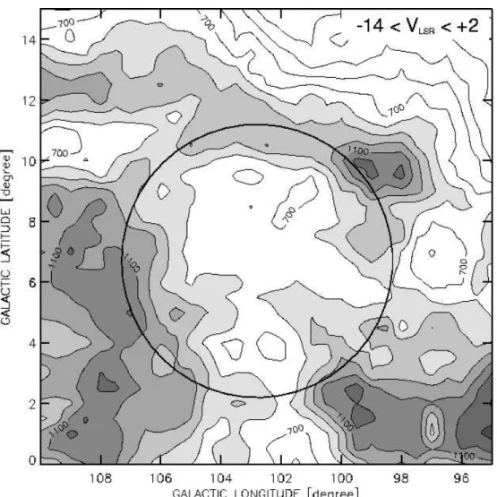
3.5 the hydrogen emission integrated between −14kms⁻¹ and +2kms⁻¹. The figure shows a well-defined closed ring around the low emission region l = 101ô to l = 105ô, b = +2ô to b = +2ô, a result also published by SVSG and by Patel et al. (1998).

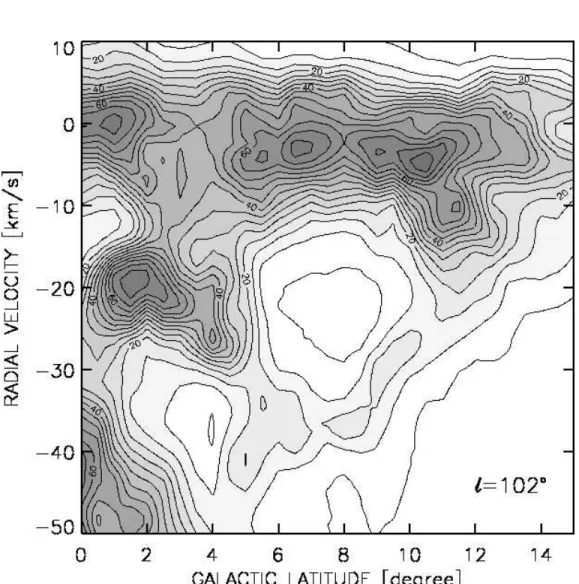
An inspection of the HI maps of Fig. 3.3, 3.4 reveals loop structures in several velocity regimes. The most prominent ring structure, with sharp inner edge in the direction of the Cepheus Bubble, appears in the V_lsr = [−14,−10]kms⁻¹ range. A similar ring-like pattern is clearly recognizable at more negative velocities as well. Between −26kms⁻¹ and −14kms⁻¹, Fig. 3.3 shows a low emission area (‘hole’), bounded by stronger HI emission regions, and the whole structure extends over about parallel to the galactic plane. Although the center of this higher negative velocity hole (l ' 103^o, b ' +8^o) is at slightly higher galactic latitude than that of the ring in Fig. 3.5, the transition between these two loop structures is contin- uous in the velocity space (Fig. 3.3, 3.4), providing a strong evidence for their physical link. At even higher negative velocities (V_LSR ' −26kms⁻¹) the upper boundary of the hole is fragmented, and the loop structure is no longer visible. The fragments are, however, still recognizable at more negative velocities, roughly following the trend that fragments of higher negative radial velocities appear closer to the center of the former ring. At V_LSR ' −30kms⁻¹ even these fragments disappear. The interpretation of these results in terms of an expanding shell is given in Sect. 3.2.3.

(36)

Figure 3.3: HI 21 cm maps toward the Cepheus Bubble in the [−38,−14]kms⁻¹velocity range, integrated over 4kms⁻¹ intervals. The lowest contour corresponds to 40 Kkms⁻¹.

(37)

Figure 3.4: Continuation of the previous Figure in the [−14,+10]kms⁻¹ velocity interval.

(38)

Figure 3.5: HI 21 cm intensity integrated between -14 and +2 kms⁻¹. The lowest contour is 300 Kkms⁻¹, the contour interval is 100 Kkms⁻¹. The circle around the low emission region marks the approximate outer boundary of the infrared ring.

(39)

So far we identified the significant cloud complexes related to the Cepheus Bubble by visual inspection of the HI maps. This method, however, is not automatic, can be somewhat subjective, and works less efficiently in regions where the resolution of the kinematic distances, resulting from the differential rotation of the Galaxy, is poor (like in the Cepheus region which is close to the l = 90^o tangent point). Visual inspection may also fail to identify structures which extend over very large radial velocity ranges due to internal and/or peculiar motions. In the next subsection we use a multivariate statistical method for identifying the main structures in the data cube representing the Cepheus Bubble, free from subjective bias.

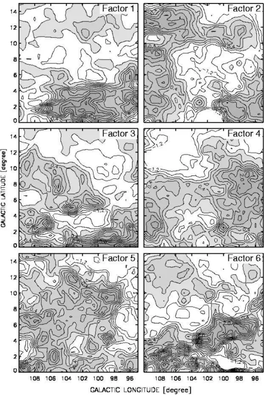
Multivariate analysis of the HI channel maps The positional and velocity data of the neutral hydrogen form a data cube {l, b, v}. We assume that the HI emission is optically thin, and the observed channel maps are weighted superpositions ofkcomponents which represent the main hydrogen cloud complexes, i.e.:

I_i =

Xk j=1

a_ijF_j i= 1, . . . , n (3.2)

whereI_i, a_ij and F_j are the measured intensities in the channel maps, the weighting coefficients, and the contributions of the components, respectively, and n is the number of the channel maps. Normally, we may assume that k < n. Description of the observed variables by linear combination of hidden variables (factors) is a standard procedure of multivariate statistics.

We make the assumption that the correlation between theF_j components is negligible. This assertion enables us to apply the principal components analysis (PCA) for finding the number of significant components (factors) and their numerical values, using standard techniques implemented in statistical software packages. The PCA represents the observed variables (T_b∆v values in our case) as linear combinations of non-correlated background variables (principal components). We note that although PCA is often used for finding the factors, there are many other techniques for obtaining a factor model.

PCA and factor analysis represent two different procedures, strongly related but not identical.

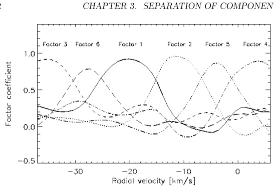
PCA obtains the factors by solving the eigenvalue equation of a matrix built up from the correlations of the observed quantities. The components of the obtained eigenvectors serve as coefficients of the factors (the significant principal components in this technique) in the equation given above. The eigenvaluesλ1, . . . λngive some hint for the ‘importance’ of the corresponding components. The λ_i/^Pⁿ

j=1 and ^Pⁿ

j=1λ_i/ ^Pⁿ

j=1 ratios indicate what percentage of