B Y
J. S H E R M A N
Philadelphia Naval Shipyard, Philadelphia, Pennsylvania
CONTENTS
Page
1. Statistical Analysis Applied to Spectrographic Measurements 502
1.1. Introduction 502 1.2. Generalities 503
1.2.1. Theory of Probability and Random Variate . 503
1.2.2. Statistical Inference 505 1.2.3. Tests of Significance and the Null Hypothesis 508
1.3. Practical Applications 511 1.3.1. Design of Experiment 511 1.3.2. Factorial Experiments. Interaction 512
1.3.3. Types of Design . . . 518
1.4. The Interrelationship of Two Variables 523
1.4.1. Introduction 523 1.4.2. The Straight Line with Random Dependent Variate 525
1.4.3. The Straight Line with Independent Variate Determined Experimentally . 527
1.4.4. The Straight Line with Both Variates Random 528
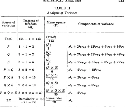
1.5. Analysis of Variance. Computation 530
1.5.1. Introduction 530 1.5.2. Complete Balanced Experiment for Means 530
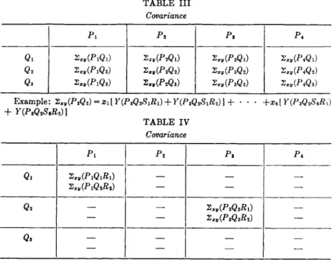
1.5.3. Complete Balanced Experiment for Regression (Covariance)
Analysis. Qualitative Interpretation of Effects 534 1.6. Computation. General Procedure for Orthogonal Comparisons.
Reduction to Single Degrees of Freedom 542
1.6.1. Introduction 542 1.6.2. Orthogonal Comparisons 543
.1.6.3. Two Effects. Interactions 547
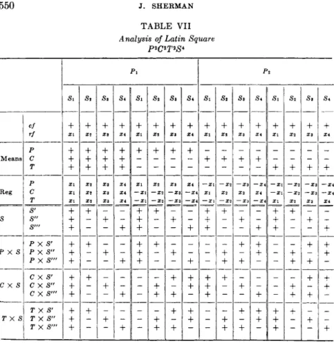
1.6.4. Latin Square 547 1.6.5. Regression or Covariance Analysis 548
1.6.6. Latin Square with Regression 549 1.7. Computation. Miscellaneous 549
1.7.1. Discriminant Functions 549 1.7.2. Dilution Correction 552
* The opinions expressed in this chapter are those of the author, not of the Navy Department.
501
When any scientific conclusion is supposed to be proved on experimental evidence, critics who still refuse to accept the conclusions are accustomed to take one of two lines of attack. They may claim that the interpretation of the experiment is faulty, that the results reported are not in fact those which should have been expected had the conclusion drawn been justified, or that they might equally well have arisen had the conclusion drawn been false. Such criticisms of interpretation are usually treated as falling within the domain of statistics.—The Design of Experiments, R. A. Fisher 1. ST A T I S T I C A L A N A L Y S I S A P P L I E D T O SP E C T R O G R A P H S M E A S U R E M E N T S
1.1. Introduction
T h i s c h a p t e r will be concerned with t h e statistical approach t o t h e e v a l u a t i o n of t h e precision of controlled physical m e a s u r e m e n t s or experiments. T h e problem will be considered as being twofold; (1) t o express precision in an objective form, usable for prediction a n d (2) t h e use of precision estimates as a guide for a methodical procedure t o e v a l u a t e t h e contributions of t h e various experimental factors t o t h e t o t a l
" e r r o r . " I t is impractical t o develop a rigorous statistical t h e o r y in this discussion. W h a t will be presented should be considered as a kind of justification or explanation of t h e general arithmetical methodology.
N o m a t h e m a t i c a l proofs or derivations will be given. While t h e symbols will be given d e n o t a t i o n s peculiar t o spectrography a n d spectrographic procedures, it should be clear t h a t a n y other consistent a n d analogous set of meanings will do equally well.
Page
1.8. Tests of Significance 552 1.8.1. The Normal Deviate 553
1.8.2. Student's t 553 1.8.3. Chi-Square 554 1.8.4. "F," Z, or Variance Ratio Test 554
1.9. Interpretation of the Analysis of Variance 556
1.9.1. Total Mean Square 556 1.9.2. Comparison of Mean Squares 557
1.9.3. Homogeneity of Variance 558
1.9.4. "F" Test 559 1.10. Prediction. Precision 561
1.11. Conclusion 564 2. Numerical Examples 566
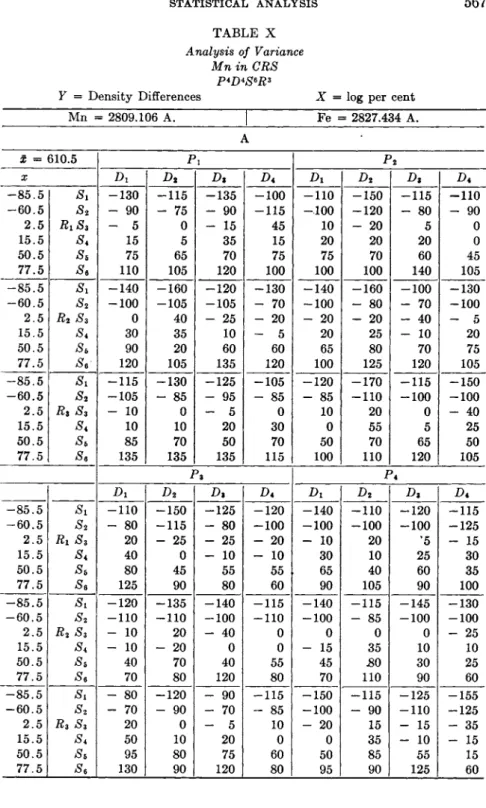
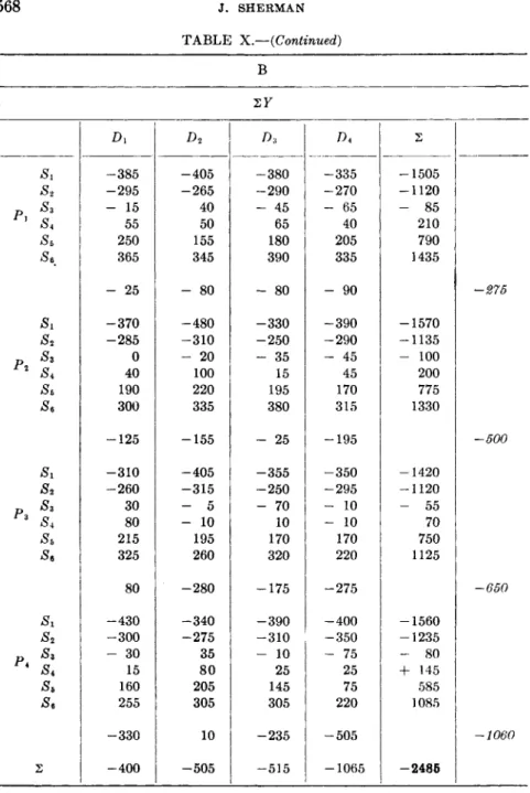
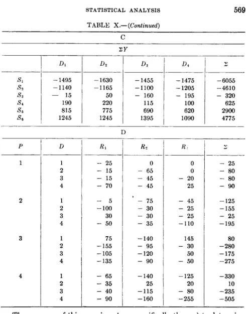
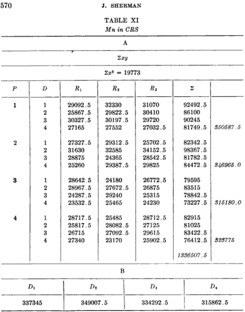
2.1. Determination of Manganese in Stainless Steel (CRS). 566
Statistical Analysis 569 Appendix. Orthogonal Partition into Single Degrees of Freedom 581
2.2. Discriminant Functions. Ni in CRS 583 2.3. Regression. Two Random Variates 584 2.4. Comparison of Microphotometer and Repetition Error 584
2.5. Plate Calibration 585 2.6. Effect of Excitation on Analytical Curve 587
2.7. Source Stability 588
References 589
1.2. Generalities
1.2.1. Theory of Probability and Random Variate. T h e concepts of probability a n d of t h e r a n d o m variable h a v e undergone m a n y transfor- mations in their historical development a n d u n d o u b t e d l y are still unsatis- factory to m a n y minds. On the one h a n d there is t h e intuitive approach in which probability is considered as having the connotation of " c h a n c e "
or " e x p e c t a t i o n . " T h u s probability has been defined as t h e measure or degree of rational belief. T h e r a n d o m variable has been similarly asso- ciated with the notion of haphazardness, or randomness, such as is observed in the usual affairs of life or in t h e erratic fluctuations in repeated physical measurements. This behavior is contrasted with the strictness of the relation between the variables in an algebraic formula say in an exact law of dynamics or in the law of constant proportions in chemistry, despite the observed fluctuations in a n y measurements based on these laws. Somehow or other, t h e ever-present fluctuations were associated with h u m a n fallibility, a n d considered, in physical science, as necessary, unpleasant concomitants t o t h e search for t r u t h , all efforts to minimize them notwithstanding. Indeed one would rather not discuss them, except as something to be abolished. While these concepts m a y be esthetically satisfying, they are hardly capable of q u a n t i t a t i v e formula- tion. A less subjective concept of probability is t h a t of frequency, in the sense of vital statistics. Certain regularities are observed in the behavior of large n u m b e r s of similar biological individuals, considered as a group:
such as height, weight or longevity even though little m a y be definitely asserted about an individual.
During the 18th century, a mathematical theory of probability was developed by extending the notion of regularity of averages of large numbers, particularly to the problems connected with t h e ordinary games of chance. In these games, the results t h a t are a priori possible m a y be arranged in a finite n u m b e r of cases supposed to be perfectly symmetrical, such as t h e cases represented by t h e 6 sides of a die, t h e 52 cards in an ordinary pack of cards, etc., and the results of any event analyzed according to combinatorial theory. These considerations led t o t h e famous principle of " e q u a l l y possible c a s e s " which was explicitly stated and extensively developed by Laplace. According to this principle, a division into "equally possible" cases is conceivable in a n y kind of observations, and t h e probability of an event is t h e ratio between t h e n u m b e r of cases favorable to t h e event a n d t h e total n u m b e r of possible cases. T h e weakness in this concept is a p p a r e n t . There is no indicated mechanism to decide whether two cases are equally possible or not.
Moreover it seems difficult, a n d to some minds even impossible, to form
a precise idea just how a division into equally possible cases could be m a d e with respect to observations not belonging to the domain of games of chance, or to apply t h e principle to experimental or physical observations.
On t h e other hand, t h e modern mathematical approach, influenced by the general tendency t o build any mathematical theory on an axio
matic basis, makes a clean break with intuition a t the very beginning.
T h e practical justification of t h e approach is based on t h e power a n d use
fulness of the derived results. E v e n t h e postulation of t h e existence of definite limits to frequency ratios is avoided and the probability of an event is considered simply as a n u m b e r associated with t h e event. T h e axiomatic development leads to a theory of probability t h a t is essentially a theory of measure in some special sort of function space. For example, consider a set function P(S) defined for sets, S, in t h a t space a n d satisfy
ing the following three conditions:
(a) P(S) is non-negative; P(S) > 0 (b) P(S) is additive:
P(Si + S2 + ' · · = P(S0 + P(S2) + · · · (for disjoint sets, S, i.e., SUSV = 0, u τ* v)
(c) P(S) is finite for a n y bounded set, S.
Hence if, for Si contained in S2)
P(Si) < P(S2) and P(0) = 0,
then, to a n y set function P(S) defined as above, there corresponds a non-decreasing point function, F ( z ) , such t h a t for any finite or infinite interval (a, 6),
F(b) - F(a) = P(a < ξ < b)
If P(R) = 1, where R is t h e entire space under consideration, then Ρ is termed a probability function, F a distribution function, and ξ a random variable. T h e mathematical theory develops from there on.
I t is indeed a far step from such abstract concepts to intuitive prob
ability However, analogously, while for purposes of elementary trigonometry and surveying, or other simple engineering needs, it is sufficient to define sin θ as the ratio of the side opposite the angle Θ, in a right-angle triangle, to the hypothenuse, for analytical purposes a more
βΖ 0 5 β7
appropriate definition is sin θ = θ — ^ + ^ — ^ + · · · . I t is also difficult to see the right-angle triangle in this expression, yet the defined function reduces to t h a t chosen for the triangle.
1.2.2. Statistical Inference. Extensive application has been m a d e of probability theory t o t h a t section of statistical inference t h a t is of interest in this discussion, namely t h e theory of errors. I t is a m a t t e r of common experience t h a t repeated measurements under apparently identical con
ditions are n o t identical, for example t h e measurement of Δ log / of a certain line pair under closely controlled conditions. Indeed, if the measurements were identical, or even within the least count of the measuring instrument (densitometer) there would be no statistical prob
lem. T h e connotation of " e r r o r , " then, is not t h a t of a mistake, either objective or subjective, b u t of an unavoidable fluctuation in repetitive measurements. These fluctuations are called random, in spite of t h e fact t h a t we are unable t o give a precise physical interpretation to the term. This situation is not entirely incompatible with a deterministic point of view, since it is realized t h a t slight, undetectible changes in the initial or intermediate conditions of an experiment m a y show u p in an exaggerated form as fluctuations in the terminal result. On the other hand, there is no question of essential theoretical indeterminancy as in t h e q u a n t u m theory. However, in spite of the irregular behavior of individual results, t h e average values of long sequences of repeated
" r a n d o m ' ' measurements show striking regularities. Accordingly, the conjecture is m a d e t h a t to an event Ε connected with a random experi
m e n t (deviation of Δ log I from the true value), it is possible to ascribe a n u m b e r Ρ such t h a t in an infinitely long series of repetitions of the random experiment, the frequency of Ε will be equal to P. This con
jecture is of course not capable of mathematical or even experimental proof, since it is impossible to perform an infinitely long sequence of measurements. However, the assumption is the typical form of statis
tical regularity which constitutes the empirical basis of statistical theory.
Then, in an extended series of measurements, under controlled condi
tions, on t h e Δ log / of a certain line pair, t h e frequency of t h e errors, or deviations from t h e true value, for any range of deviations will approach a fixed value. I t should be noted t h a t t h e application is m a d e t o a range of deviations since Ρ is a set function, a n d not to a single or individual value of t h e derivation. Indeed, the value of Ρ for any individual value of the deviation is zero, on t h e assumption of the continuity of t h e values of t h e error. This m a y be concealed in a n y physical measurement due to t h e least count of the measuring instrument, δ, since then a single measurement really corresponds t o the range of ± δ.
I t is now further assumed, in keeping with general physical evidence, t h a t t h e errors of s p e c t r o g r a p h s measurements approximately follow a normal or Gaussian distribution. While t h e precise specific formulation of this distribution is not i m p o r t a n t it m a y be stated t h a t it implies t h a t
the errors are symmetrically distributed around the true value or zero, and t h a t large errors occur less frequently t h a n small ones. Explicitly,
where £ is the random variate, i.e., error, m is the true value of the varia
ble, (here m = 0), σ is a measure of the spread of the errors (standard deviation), defined as follows, σ2 = lim - / (£,· — ra)2 where η is the n u m b e r of measurements, and (λ, <») is the range of the variate con
sidered. I t is t o be noted t h a t the function Ρ is completely determined, for any λ, if two parameters, m and σ are known.
However, t h e formulation of the distribution, even if only assumed, does not lead very far in itself. T h e parameters ra, σ are not known and indeed can never be known as the results of any finite experiment no m a t t e r how extended. Accordingly, any experiment is considered to be a sample of all possible measurements, or population, of the kind under consideration. Actually even an infinite series of measurements would not be quite enough, since the normal distribution assumes t h a t the average or arithmetic mean of the measurements, lim - > χ; is the true value, and any knowledge of the difference between ra and the true value is extra-experimental a n d cannot be detected. However, neglect
ing this point, it m a y be seen t h a t t h e problem is really t h a t of estimating ra and σ from the results of experiments of finite length. This is quite a difficult problem considered either from experimental or theoretical aspects. One m u s t be assured of the representation of the sample, i.e., whether it is truly random or biased. I t appears almost too much to expect t h a t any experiment of reasonable magnitude will contain the true proportionality of elementary disturbing factors, consequently a major p a r t of t h e theoretical effort m u s t be devoted t o tests for random
ness or quality of representation of the sample experiment. Sampling theory is divided into two parts, t h a t of large samples and small samples.
I n large sample theory it is assumed t h a t t h e experiment exhibits an effectively true and complete state of affairs, in miniature, and t h e p a r a m eters m a y be computed directly as if t h e entire infinite population were available. Then, after the parameters have been estimated, tests m a y be devised t o see whether t h e distribution is truly normal, or whether another t y p e of distribution would fit t h e facts more precisely. I t m a y reasonably be assumed t h a t large samples, in this sense, will not be
η
η
ι —
available in s p e c t r o g r a p h s procedures. T h e theoretical problem in small samples is the relation between t h e parameters as computed from the samples, or statistics, a n d t h e parameters of t h e assumed infinite parent population or true values of the parameters. I n other words, the prob
lem is t h a t of the distribution of sample statistics, the samples being taken from a population of an assumed normal character. I t will be evident t h a t if a sample is not r a n d o m a n d nothing precise is known a b o u t the n a t u r e of t h e bias operating when it was chosen, very little can be inferred from it a b o u t t h e p a r e n t population. Certain conclusions of a trivial kind are indeed always possible, for instance, if one were to t a k e 10 turnips from a population of 100 a n d find t h a t they weigh 10 pounds altogether, t h e m e a n weight of turnips in t h e pile m u s t be greater t h a n
XV of a p o u n d ; b u t such information is rarely of value, a n d estimations based on biassed samples remain very m u c h a m a t t e r of individual opinion a n d cannot be reduced to exact a n d objective terms.
Let it be considered w h a t is m e a n t by estimation in general. I t is known or assumed as a working hypothesis t h a t the parent population is distributed in a form which would be completely determined if t h e value of some p a r a m e t e r θ were known (in t h e one dimensional case). A sample of values [Xi, . . . , Xn} are given. I t is required to determine, with t h e aid of t h e X'a, a n u m b e r which can be taken as the value of 0, or a range of numbers which can be t a k e n to include t h a t value. Now a single sample, considered b y itself, m a y be rather improbable and any estimate based on it m a y therefore differ considerably from the true value of 0. I t appears, therefore, t h a t one cannot expect t o find any method of estimation which can be guaranteed t o give a close estimate of 0 on every occasion and for every sample. One m u s t be content with the formulation of a rule which will give good results " i n t h e long r u n , "
or " o n the average," or which has " a high probability of success,"
phrases which express t h e fundamental fact t h a t one has to regard the method of estimation as generating a population of estimates and to assess its merits according t o the properties of this population. As a rule the estimates are given as functions of n, t h e size of t h e sample, and all t h a t is t o be expected is t h a t t h e estimate will converge to t h e true value (that of t h e p a r e n t population) as η increases indefinitely. E v e n t h e problem of convergence is intricate. Convergence is an analytical sense has been quite well understood since t h e time of Cauchy, b u t in prob
ability theory t h e classical notion m u s t be modified, since for a r a n d o m variate £, £n cannot be expressed as a function of n. Indeed, a prob
ability Ρ = 0 does not mean the event never occurs since it is a char
acteristic of the integration process (Lebesgue) t h a t a set of measure zero m a y be arbitrarily added or subtracted from t h e set of t h e inde-
pendent variable, η. Ρ = 0 means only t h a t the event will occur, say, no more t h a n in a few isolated instances in an infinite run. A similar condition prevails with regard to certain occurrence when Ρ = 1, i.e., the event m a y not occur in a few isolated instances in an infinite run. (The term few is used in a relative sense.) While the discussion has been con
cerned with a one parameter, or one dimensional distribution, the exten
sion to more dimensions is, a t least, logically clear.
NOTE: A logical objection has sometimes been expressed concerning the applica
bility of the normal distribution to error theory, since, it is argued, very large errors are theoretically feasible although they are certainly not practically possible. The argument is really concerned with the conceptual difficulty in the application of the limit of an infinite mathematical process to empirical data and simultaneously con
sidering the application of the process in a term-wise manner. Discussion of diffi
culties of this type go back at least to the time of Zeno. All that need be said at this time is that very large errors are very improbable, the larger the error the greater the improbability, and that any mathematical process must be a convergent one, in some sense, before it can be used.
1.2.3. Tests of Significance and the Null Hypothesis. F r o m w h a t has been said before, it is seen t h a t t h e central problem in sampling theory is not only t o estimate t h e population parameters from t h e sample statistics b u t also to estimate the closeness of the estimations. T h e two most important parameters to be estimated, particularly for normal dis
tributions, are the mean or average value and the spread of t h e values around t h e average. T h e spread is t o be measured by t h e dispersion or variance, i.e., σ2 = - / (Γ» — y)2 where y is the m e a n and Ft the indi
vidual observation. For ordinary functional relations, the two p a r a m eters y a n d σ2 would be estimated from two sets of independent observa
tions, i.e., samples. However, this simple procedure is n o t sufficient for probability theory.
I t has been emphasized t h a t no mathematical theory deals directly with objects of immediate physical experience. T h e m a t h e m a t i c a l theory belongs entirely to t h e conceptual sphere a n d deals with purely abstract objects. T h e theory is, however, designed to form a model of a certain group of phenomena in the physical world a n d t h e abstract objects a n d propositions of t h e theory h a v e their counterparts in certain observa
ble things a n d relations between things. T h e concept of mathematical probability has its counterpart in certain observable frequency ratios.
Accordingly it is required t h a t , whenever a theoretical deduction leads to a definite numerical value for t h e probability of a certain observable event, the t r u t h of t h e corresponding frequency interpretation should be borne out by observation. Thus, when the probability of an event is
very small, it is required t h a t in t h e long run t h e event should occur a t most in a very small fraction of all repetitions of t h e corresponding experi
ment. Consequently, one m u s t be able t o regard it as practically certain t h a t , in a single performance of t h e experiment, t h e event will not occur.
Similarly, when t h e probability of an event differs from 1 by a very small a m o u n t , it m u s t be required t h a t it should be practically certain t h a t , in a single performance of t h e corresponding experiment, t h e event will occur. In a great n u m b e r of cases, t h e problem of testing t h e agreement between theory and fact presents itself in t h e following form. One has a t one's disposal a sample of η observed values of some variable, a n d it is required to test whether this variable m a y reasonably be regarded as a r a n d o m variable associated with a certain distribution. In some cases the hypothetical distribution will be completely specified, for example a normal distribution with m = 0 and σ2 = 1. In other cases, it is required to test t h e hypothesis t h a t the sample might have been drawn from a population with this distribution. One begins by assuming t h a t t h e hypothesis to be tested is true. I t then follows t h a t t h e distribution function, F*, of t h e sample m a y be expected to approximate t h e distribu
tion function of t h e population, F, when η is large. Let some non-nega
tive measure of t h e deviation of F * from F be defined. This m a y , of course, be m a d e in various ways, b u t a n y deviation measure D will be some function of t h e sample values and will t h u s have a determined sampling distribution. B y means of this sampling distribution, one m a y calculate t h e probability P(D > D,0) t h a t t h e deviation D will exceed a n y given n u m b e r Do. This probability m a y be m a d e as small as one pleases by taking D0 sufficiently large. Let D0 be chosen so t h a t P{D > Do) = e , where e is so small t h a t one is prepared t o regard it as practically certain t h a t an event of probability e will not occur in a single trial. T h e value of D is then computed from the actual sample values.
T h e n if D > Do, it means t h a t an event of probability e has presented itself. However, the hypothesis was t h a t such an event ought to be practically impossible in a single trial, a n d t h u s one m u s t reach the conclusion t h a t the hypothesis has been disproved by experience. On the other hand, if D < D0, one should be willing to accept t h e hypothesis as a reasonable interpretation of the data, at least until further evidence is presented. If in t h e actual case, D > Do, it is said t h a t t h e deviation is significant. Tests of this general character are called tests of signifi
cance. T h e probability €, which m a y be arbitrarily fixed, is called t h e level of significance, and t h e higher t h e probability e the lower the signif
icance level. I n t h e case where t h e deviation measure D exceeds the significance level one m a y regard t h e hypothesis as disproved b y experi
ence, a condition by no means equivalent to logical disproof. E v e n if
the hypothesis were true, the event D > Do, with a probability c, m a y occur in an exceptional case. However, when e is sufficiently small, one m a y be practically justified in disregarding this possibility. On the other hand, the occurrence of a single value D < D0 does not provide a proof of the t r u t h of t h e hypothesis. I t only shows t h a t , from the point of view of t h e particular test, the agreement between theory and observa
tion is satisfactory. Before a statistical hypothesis can be regarded as practically established, it will have to pass repeated tests of different kinds.
Let a sample of spectrographic measurements, Δ log / for a certain line pair be given. I t is required to justify the hypothesis t h a t the deviations or errors are normally distributed, say around zero. I t has been seen how this question m a y be answered by a properly chosen significance test. On the other hand, let it be supposed t h a t the general character of the distribution is known from previous experience and information is required concerning the values of some particular charac
teristics of the distribution. For example, let a comparison be m a d e between effects of two electrode shapes on the error. T h e error distribu
tions, i.e., the probability or frequency of an error or deviation within a certain range, are assumed known for each sample form and they are assumed to be nonidentical. Then the question m a y be asked whether the difference is due to random or sampling fluctuations or is significant, i.e., indicative of a real difference between the probabilities. In such cases it is often useful to begin by considering t h a t there is no difference between the two cases (electrode shapes), so t h a t in reality all the sample observations come from the same population. This is called the null hypothesis. This being assumed, it is often possible to construct sig
nificance tests for the difference between the means, or other charac
teristics. If the differences exceed certain limits, t h e y will be regarded as significant and one m a y conclude t h a t there is, practically, a real difference between the cases, i.e., effect of electrode forms; otherwise the differences will be ascribed to random or sample fluctuation. I t should be borne in mind t h a t a significant difference merely disproves the null hypothesis a t a certain probability level in a logical sense, and does not logically prove the existence of a factual difference between the effects of t h e two cases.
There are two kinds of errors or incorrect conclusions t h a t m a y be drawn concerning the significance of a difference in effect, to carry out the previous example, of the electrode forms. Let the null hypothesis be indicated as Ho, i.e., the difference between the electrodes is merely a random or sampling effect, and let Hi be an alternative hypothesis t h a t need not be specified. Then an error of the first kind is committed when
H0 is rejected when it is true, i.e., it is decided t h a t " t h e difference between the electrode forms is r a n d o m " is n o t true when it actually is.
An error of t h e second kind is c o m m i t t e d when H0 is accepted when Hi is true. T h e probability of an error of t h e first kind m a y be indicated by a a n d t h a t of an error of t h e second kind by β. T h e choice of tests should be of course in t h e direction of minimizing both a a n d β. Under most practical conditions, it is impossible to m a k e t h e m both arbitrarily small, and the decision is usually m a d e by choosing a, then devising a test to minimize β. For a fixed sample size, under certain mathematical conditions, β is a single-valued function of a, and if a is small, β(α) is in general large, a n d if a is large β(α) is small. T h e choice of a or β should be influenced by the relative importance of the two kinds of errors.
1.8. Practical Applications
1.3.1. Design of Experiment. Fortunately, at least for t h e sake of expediency, a theoretical development such as discussed above is not necessary for t h e application of the statistical methods to experimental d a t a t h a t will be considered. I t m a y simply be assumed t h a t m a t h e matical tests of significance have been devised and, more or less, gen
erally accepted. However, it should be realized t h a t in order to apply these tests in a proper manner, it is often necessary t h a t the experimental d a t a be obtained in a certain way. T h e arrangement of t h e course of an experiment so t h a t statistical tests or computations m a y be subsequently performed on t h e d a t a m a y be called the design of an experiment. I t is i m p o r t a n t t h a t an experiment be carefully considered from this point of view before t h e d a t a is accumulated or measurements made.
Accordingly, t h e practical course of a statistical study m a y be divided into three p a r t s ; (a) arrangement, or design of the experiment, with regard to t h e variables or factors being studied, (b) computation of cer
tain statistics a n d (c) determination of significance by reference to certain tables.
T h e general approach will be t h a t of variance analysis, with a n d with
out reduction for regression, while significance will be determined by reference to the " F " or chi-square test (the exact meaning of these terms will be developed later). I t will be observed t h a t the computation is purely arithmetical, and m a y be rather extensive so t h a t a modern elec
trical computing machine with automatic multiplication and division is practically a necessity. Some p a r t s of the computation will yield results useful in themselves, independent of their significance, for example, the slope of a calibration or working curve, the equivalence point, etc. T h e tables for determining significance m a y be used in a similar manner. In all cases, t h e y will associate the value of the statistic with the probability
t h a t it is as large as it is purely as r a n d o m happening due to sampling, i.e., based on the null-hypothesis. While t h e choice of significance levels is more or less arbitrary and a m a t t e r of personal judgment, for the sake of uniformity it will be assumed t h a t
(a) Ρ > .05, definitely when Ρ > .10, will be interpreted as non
significant,
(b) Ρ < .01, definitely when Ρ < .001, will be considered significant.
Intermediate values, i.e., .01 < Ρ < .05 will be considered indecisive a n d j u d g m e n t reserved until further experimentation has been effected.
I t need hardly be repeated, b u t the significance determined from these tables is a statistical, not a physical or engineering, test and t h a t evalua
tion from the experimental side is always necessary.
In concluding these general remarks it m a y be stated t h a t not all significance tests are equally good since consideration m u s t be given to the rapidity of their convergence (in probability) with increasing η or decreasing 1/n (efficiency), and to the dispersion or spread of their dis
tribution functions around their central or limiting value. I t is suggested t h a t the reader consult the references for a full mathematical t r e a t m e n t of the preceding discussion.
1.3.2. Factorial Experiments. Interaction
(1) Introduction. In order to understand fully the reasoning govern
ing the differences between suitable and unsuitable arrangements of an experiment it is of course necessary to understand the m a n n e r in which the computations on the experimental d a t a are to be performed, and vice versa. However, since a beginning m u s t be made, a few general statements, introducing the subsequent t r e a t m e n t , will be a sufficient introduction.
Let F represent the dependent variable, t h a t is Ft is the ith measure
m e n t or estimation of t h e density of a line, t h e Δ log / of a line pair or the per cent of an element in some material being analyzed. Then Ft is a function of recognized main experimental factors, Ft = F , ( P , Q, R, S, . . . ), where the independent arguments P, Q, R, S may, for present purposes represent such factors as photographic plates, the various com
ponents of an excitation system, electrode shape, line pairs, densitometer sensivity, etc. T h e error in Yi} Yi — y where y represents the true value of F , depends on the combined result of the errors or uncontrollable fluctuations in the response of P, Q, R, S, . . . . I t will be assumed, until proved otherwise in some manner, t h a t the random fluctuations or errors attributable to each of P , Q, R, S, follow a normal distribution law.
There are several reasons for assuming a normal distribution for the
errors in the parent population (of t h e independent arguments). I n the first place, for error theory, the normal law is nearly always an excellent approximation. F u r t h e r m o r e , investigations on non-normal popula
tions have shown t h a t even considerable departures from normality do not produce appreciable changes in m a n y i m p o r t a n t deductions based on the normal law. I t has also been established t h a t statistics such as the mean, computed from samples drawn from a non-normal p a r e n t popula
tion are often m u c h more normal t h a n t h e population itself. T h e degree of necessity for normality in t h e p a r e n t population really depends on t h e character of t h e distribution of t h e significance tests employed. In general, for present purposes, a n y bell-shaped distribu
tion with a h u m p in t h e middle and tapering off a t b o t h sides will be satisfactory as a good approximation. There are some very i m p o r t a n t consequences of this assumption of normality. I n t h e first place, it follows, rigorously, t h a t t h e errors in F are normally distributed. Let y stand for the t r u e value of F , then t h e measure t o be used for t h e spread, or error, in a n u m b e r of measurements of F will not be, for example, ί ^ \ Yi: — y\, b u t the variance, σ2 = ί ^ (Yt: — y)2. T h e square root of this q u a n t i t y , σ, is called t h e s t a n d a r d deviation. I t follows from the normal law, if no systematic errors are present, t h a t t h e m e a n of t h e parent population would be t h e t r u e value of t h e q u a n t i t y being meas
ured. (The effect of a systematic error would be to displace the mean of the p a r e n t population of observations t o one side or t h e other of the true value, a n d t h e correction, if ever isolated, can be added t o t h e mean of the p a r e n t population to give the true value. T h e effect of a system
atic error cannot be isolated or even detected by t h e theory of t h e random variable.) I t also follows t h a t t h e sample m e a n is t h e best approxima
tion to the population mean. I t m a y be shown t h a t t h e variance of sample means, σ^2 = ί σ2, where y will from now on indicate t h e mean value, σ^2 the variance of the y (as a sample statistic) a n d σ2 is t h e variance of t h e individual measurements. T h e improvement in precision involved in t h e use of a mean of multiple measurements" has long been recognized.
Indeed there are only two ways intuitively used to improve t h e other
wise unsatisfactory precision of m e a s u r e m e n t s : (1) to modify or improve the experimental conditions a n d (2) to use t h e mean-of repeated observa
tions. Particular attention should be paid to the condition of inde
pendence of P, Q, R, . . . . In the model of the m a t h e m a t i c a l theory of probability, independence has the following meaning. If t h e distribu
tion functions of t h e r a n d o m variables Q and R are Qi(u) a n d Ri(v), then the distribution of Y(u, v) = Qi{u)R\(v). For a normal distribution
this implies συ2 = aQl2 + σβ χ 2. Empirically, independence m a y be assumed for two factors Q and R if one can be changed without affecting the other.
If the conditions of successive random experiments are strictly uniform, the probability of any specified event, for example the magnitude of error, connected with the nih experiment cannot be supposed to be in any way influenced by the η — 1 preceding experiments. This implies t h a t the distribution of the random variable associated with the nth experi
ment is independent of any hypothesis made with respect to the value assumed by the combined preceding η — 1 variables. A sequence of repetitions of a random experiment showing a uniformity of this charac
ter will be denoted as a sequence of independent repetitions. When nothing is stated to the contrary, it will always be assumed t h a t any sequence of repetitions considered will be of this type.
T h e purpose of a considered arrangement of the factors in an experi
ment, or experimental design, is to insure as efficient an independent repetition of the effects of the principal factors, or main effects, in order to make full use of the improvement in precision involved in the use of the mean of multiple observations and as far as possible, to cancel out systematic errors.
(#) Factorial Experiments. T h e classical ideal of experimentation is to have all independent variables but one constant. It is frequently not recognized t h a t this m a y sometimes be far from ideal, for in order to obtain a fair assessment of the effects of varying the particular variable selected one must also allow the others to vary over their full normal range. If they were to be held constant, it would necessarily be at arbitrary value. Thus, varying factor Q, say secondary voltage, from its normal value, Q\, to another value Qz, m a y affect one change in the dependent variable Y, when factor R, say electrode form, is at Rh but m a y quite conceivably induce another change when factor R is at R2. This is not incompatible with the notion of independence, b u t introduces a new variable, namely the interaction of Q and R, written as Q X R.
The factorial experiment is designed to detect this type of effect as well as for maximum efficiency, i.e., to give the maximum a m o u n t of informa
tion about the system being experimented upon for a given amount of effort. I t is ideally suited for experiments whose purpose is to m a p a function, Y, in a preassigned range of values of the independent variables.
(a) Three factor experiment:
Consider an experiment to investigate Y as dependent on three factors, F ( P , Q, R). (For- specific meanings, Υ == Δ log I, Ρ = photographic plate, Q = some excitation condition, and R = electrode shape.) I t m a y be considered adequate, for the example or as a first a t t e m p t , to restrict the range of P, Q, and R to two values or levels. It should be
noted t h a t there m a y be no numerical measure of the difference between the two levels, for example R\ m a y be rods with conical top while R2 m a y be a flat surface with a graphite counter electrode. Let t h e normal value be Yi = Y(Pi, Qi, Ri). T h e classical experiment, t h a t of changing one variable a t a time, would be to obtain four observations, namely
1. Y(Ph Qi, #1) , 2. F ( P2, Qi, P i ) , 3. F ( P1 } Q2, P i ) , 4. Y(Plf Qh P2) .
T h e effect of the change i n P , i.e., (Pi — P2) r would be obtained from t h e first two measurements, the change in Q, (Qi — Q2)r would be obtained from a comparison of the first and third observation, while the change in R would be obtained from a comparison of the first and fourth observa
tion. Now it is i m p o r t a n t to observe, t h a t each of these observations would have to be repeated n o t less t h a n once, for with use of less t h a n two observations at constant conditions, it is quite impossible to form any estimate of the non-reducible experimental error, i.e., σ2, t h a t of a single observation, which would serve as a basis for comparison. With
out such a basis, it would be impossible to decide whether the observed, or apparent, difference in Y due to a change in, say, P , is real i.e., signifi
cant, or due to the errors of experiment. T h e complete set will, then, consist of four measurements repeated once, or eight measurements in all. E a c h level of each effect or factor will be given by two observa
tions, i.e., comparisons will be between one mean of two observations and another mean of two observations. N o information will be given by this type of experiment concerning the possible interaction between effects. F o r example (Pi — P2) r at R = P i m a y be appreciably different from (Pi - P2) y a t R = R2.
On t h e other h a n d in a factorial design, one would carry out all com
binations of P, Q, R, a t all levels, namely, eight observations:
(1) ( Pl f Qlt P i ) , (2) CPl f Q1} R2), (3) ( Pl f Q2, P O , (4) (Ph Q2, R2)
(5) ( P2, Qi, P i ) , (6) ( P2, Qi, P2) , (7) ( P2, Q2, P i ) , (8) ( P2, Q2, Ri) T h e n u m b e r of observations is then t h e same as in the classical design.
I t m a y m a k e it easier to grasp the meaning of the above set of com
binations if they are represented as points in the three component vector space of P , Q a n d R One m a y obtain an estimate of (Pi — Ρ2)γ by comparing t h e average of t h e P i plane with t h e average of t h e P2 plane, for although Q a n d R v a r y in each plane, the variations are equal a n d a t least to a first approximation, cancel out. T h e other main effects, (Qi — QI)Y a n d (Pi — P2) r are obtained similarly as differences in the averages of the corresponding planes.
T h e first a d v a n t a g e of the factorial design is t h a t the main effects are obtained as t h e difference between t h e means of sets of four observa-
tions. I n the classical design, these effects were obtained as differences between means of sets of only two observations. Hence t h e variance of t h e means has been cut in half with no increase in total effort.
The second a d v a n t a g e of the factorial design is t h a t it provides an estimate of the possible interactions between the main effects. T o obtain t h e interaction, for example, of Ρ a n d R, i.e., Ρ X R, one averages over Q for each P»#y, and t h u s obtains four means,
where the * in place of Q indicates a m e a n with respect to Q. Hence, the difference between the values in the top row gives Y(Pi — P2) a t R = Ri while the difference between the values in the b o t t o m row gives
Y(P\ — P2) at R = R2. T h e difference between these differences is a measure of the interaction of Ρ and R. Interactions between t h e other effects, i.e., Ρ X Q, Q X R m a y be estimated in a similar fashion. An interaction is symmetrical with respect to the component effects, i.e., Ρ X R = R X P .
Another viewpoint m a y help further to clarify the concept of inter
action. Consider the observations averaged over Q as before. T h e n F(P», Rj, *) = Pi + Rj + Pl X Rj where P , and Rj are the means of t h e respective classifications. If there were no interaction, then F ( Pt, Rj)
R
Y(Pi,Ri,*),
would equal Pi + R3. Hence Pi X Rj m a y be considered as a kind of discrepance. Dispensing with t h e restriction of two levels, consider t h e tabular values of an experiment P5R4(QX). T h e Q multiplicity is of no m o m e n t since t h e effect is averaged out
Pi P2 P 3 PA P* Σ (Mean R)R
Ri 4 18 26 38 44 130 26
R2 3 19 25 35 43 125 25
R> 6 18 24 28 39 115 23
R* 7 13 21 31 38 110 22
Σ 20 68 96 132 164 480
(Mean P ) P 5 7 24 33 41 Grand mean = 24
Transforming t h e values into deviations from t h e m e a n :
Pi 2>2 P3 7>4 Vb Σ Mean r(f)
ri - 2 0 - 6 2 14 20 10 2
r2 - 2 1 - 5 1 11 19 5 1
r% - 1 8 - 6 0 4 15 - 5 - 1
TA - 1 7 - 1 1 - 3 7 14 - 1 0 - 2
Σ - 7 6 - 2 8 0 36 68
Ρ - 1 9 - 7 0 9 17
Considering t h e interaction Ρ X R as a discrepance
p% rj = pi + rf + pi X r ,
a n d one obtains t h e interaction table
Ρ X R
Pi P2 Pa P 4 Ps Σ
Ri - 3 - 1 0 3 1 0
R2 - 3 1 0 1 1 0
Rz 2 2 1 - 4 - 1 0
R* 4 - 2 - 1 0 - 1 0
Σ 0 0 0 0 0
If there were no interaction t h e entries in t h e last table would be all zeros. F o r example, t h e expected value of p 2rz would be t h e sum of p2 + r3 = ( —7) + ( —1) = —8. Since the value of p2r3 is —6, t h e interaction t e r m P2 X Rz = 2.
(b) Higher factorial experiments:
The extension to a four-factor experiment is logically clear. If t h e factors are still t o be investigated at two levels each, P2Q2R2S2, 24 = 16 observations will be required. T h e main effects will be given by differ
ences between means of eight observations. There will be six possible first order interactions, i.e., interactions of two main effects as previously discussed, namely, Ρ X Q, Ρ X R, Ρ X S, Q X R, Q X S a n d R X S.
T o obtain t h e m one averages over the factors not indicated in t h e symbol;
thus, to obtain Ρ X Q, one averages over R a n d S. These interactions are determined as differences between means of sets of four observations.
In addition it is possible to obtain higher or second order interactions namely Ρ X Q X R, Ρ X Q X S, Ρ X R X S, a n d Q X R X S. T h e interpretation of these is simply an extension of t h a t of the first order reaction, t h u s Ρ X Q X R may be considered as the interaction of Ρ X Q and R. Interactions of any order are symmetrica! with respect to the component effects.
T h e nearest equivalent classical design would be to carry out the set of five combinations
Pi Qi P i £1 P2 Qi P i
s
lP i Q2 P i £1
P i Qi Ρ 2 .Si P i Ol P i
with a double repetition of each set, or 15 observations in all. T h e main effects \vould be determined as differences between means of sets of only three observations with no information given concerning the interactions. In the classical design, only P1Q1R1S1 is used several times, while a n y other t e r m contributes information concerning only one effect;
for example P2Q1R1S1 contributes information only concerning P , and adds nothing to the knowledge of the other factors (and of course inter
actions). In the factorial design, on the other hand, every observation is used m a n y times over, in a different manner each time
1.3.3. Types of Design
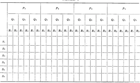
(1) Balanced Complete Randomized Blocks. T h e design of experi
m e n t implicitly considered η the preceding section is known as t h a t of balanced complete randomized blocks. T h e meaning of this is as follows:
A block is considered as the main unit of t h e experiment a n d replication of the block furnishes the measure of unassigned experimental error. For spectrographic purposes, unless otherwise indicated, a plate will repre
sent a block. T h e experiment is called balanced if the various levels of the factors are repeated an equal number of times and complete means t h a t each block, or plate, contains a full set of combinations of all levels of the factors. The term randomized refers to the r a n d o m placement of the combinations within the block, or plate; however this aspect will
be of little significance for spectrographic work since, neglecting t h e very edges of t h e plates, there are no preferred systematic arrangements within t h e plate. For example, if one wished to investigate the effect of electrode form a t four levels, E\ and excitation condition a t five levels, Cb, one would have to p u t 5 X 4 = 20 spectra on each plate, ClE\ with plate replication to an adequate amount.
This design is comprehensive a n d yields information concerning all main effects and their interactions. There are certain difficulties a n d criticisms, however, of this design t h a t are n o t trivial. First, t h e size of t h e block m a y become too great. If m a n y effects a n d m a n y levels for each effect are necessary, t h e n u m b e r of combinations m a y become too large to p u t on one plate. F o r example, CbE*Mb, where Μ represents material types, implies t h e use of 100 spectra, which obviously cannot be p u t on a single plate. Secondly, it has been found t h a t higher order interactions, say greater t h a n t h e second, usually are difficult to interpret in a physical sense a n d it m a y be felt t h a t t h e effort to compute t h e m is largely useless. More i m p o r t a n t t h a n t h e computational effort, how
ever, is t h e consideration t h a t t h e effort could be more profitably made, in t h e design, t o yield more precise estimates of t h e main effects a n d then interactions of lower order. T h e third criticism is still more serious.
Certain experimental factors, particularly those involving a time-like effect simply cannot be combined in a complete manner.
For example, suppose it is desired t o estimate t h e stability of t h e source with respect t o time. One might use two spectrographs, expose two plates simultaneously a t T\ (T = time) a n d then interchange t h e plates a n d expose t h e m a t T2. T h e experiment would be of t h e form P2T2S2 (P = plate, Τ = time a n d £ = spectrograph). (It is assumed t h a t only one plate m a y be used in a spectrograph a t a time.) Then the balanced complete set of observations would be eight in all, and arranged as follows:
(1) P i T u S , (2) PlT1S2 (3) P/YVSi (4) PJ\S2 (5) P2T1Sl (6) P27 V S2 (7) P27V>! (8) P2TiS2
Obviously (1) a n d (2) are an impossible pair, since one cannot expose one plate simultaneously in two spectrographs. I t is clear t h a t the possible arrangements are (1), (6) a n d (7), (4).
One need not be restricted to t h e denotation of plates for block.
For example, in a time study, one m a y consider all observations on one day as t h e block, or all observations on a given material, excitation con
dition, electrode form, etc.
(2) Balanced Incomplete Blocks. Accordingly, t h e experiment design m a y necessarily require modification so t h a t while t h e combination of effects a n d levels are still equally frequent, t h e blocks are n o t complete
and will no longer be exactly alike in their t r e a t m e n t s . I t is really necessary to u n d e r s t a n d the consequent mode of computation in order to discuss t h e possible designs in a critical manner, b u t some consideration will be clear. T h e i m p o r t a n t point t o consider is t h a t this design depends too m u c h on t h e combinatorial properties of t h e n u m b e r s of combina
tions of effects X levels, or t r e a t m e n t s , a n d too m a n y repetitions m a y be necessary to obtain balance.
If ν t r e a t m e n t s , i.e., effect X levels, are to be compared in blocks (assumed to be plates) of Κ spectra per plate, (K < v), t h e arrangement m u s t be such t h a t every two t r e a t m e n t s occur together in t h e same n u m b e r (λ) of plates. If r is t h e n u m b e r of repetitions, and b the n u m b e r of blocks or plates, t h e n u m b e r of spectra is rv = bk a n d λ = ^ _ ^ · Arrangements satisfying the required conditions are clearly provided by taking all possible combinations of t h e ν t r e a t m e n t s , A; a t a time, b u t if ν is at all large, t h e n u m b e r of repetitions required will be very large.
Tables are available for those arrangements requiring less t h a n 10 repeti
tions. Generally v2 t r e a t m e n t s will require (v + 1) repetitions, which m a y be considered too m a n y . However, sometimes this design m a y be p u t to effective use. Consider an experiment of form C5E2R2, where C = excitation conditions, Ε = electrode form a n d R = repetition.
Let it be assumed t h a t 16 spectra m a y be p u t on one plate. T h e plate is assumed to represent t h e block and it is known t h a t plates are not uniform in their response. Hence t h e experiment is really of t h e form PxCbE2R2, and a suitable set of combinations is Κ = 16, ν = 10, b = χ = 5, λ = 4 and τ = 8 (two repetitions on each of four plates). T h e arrangement m a y be t a b u l a t e d as follows (each e n t r y represents two spectra as repetitions).
Pi P2 Pz PA P6
CiEl CiEi CxEx CiE2
CiE* dE2 C,E2 C2EI C2E1
C2E1 C2E1 C2E2 C2E2 C2E2
C2E2 CzE\ C$E\ C3EI CzEi
CzE2 C C3E2
C,E1 C4#l C4E1 C4E2 C4E2
C4E2 C4E2 CBEI ChE\ CbEi
CbE\ cf>E2 C&E2 C^E% CbE2
This arrangement merits some study. E v e r y t r e a t m e n t is compared with every other t r e a t m e n t on three plates, any combinations of two levels of C are on one plate, Ε is repeated four times on each plate etc.
(3) Lattice Squares. I n order t o avoid t h e restriction t o t h e peculiar properties of combinations of numbers, a lattice square arrangement m a y be m a d e . T h e combinations of t r e a t m e n t s are arranged in a table a n d the rows a n d columns used as block units. F o r example, in t h e experi
m e n t CZE4, t h e t r e a t m e n t s are t a b u l a t e d
C\E\ C1E2 C\Ez C1E4 C2E1 C2E2 C2E3 C2E4 CzEi C3E2 C 3 P 3 C 3 P 4
T h e rows a n d columns are p u t on plates (seven) with a suitable n u m b e r of replicates (say t w o ) . T h e design is n o t balanced, since some com
binations, for example C1E1 a n d CiE2 are n o t compared in t h e same block or plate. However satisfactory comparisons are possible through inter
mediates, a n d with appropriate algebraic t r e a t m e n t t h e design is very efficient.
(4) Latin Squares. This design m a y be illustrated as follows. Con
sider t h e previous example on determination of source stability, a n d let the arrangement be as follows:
P i P2
$ 1 ^ 1 S2T1
S2T2 S\T2
Comparison of t h e rows will estimate t h e main effect T, t h e columns will give P , while t h e diagonals will give S. I t is t o be seen t h a t t h e interactions are confounded, t h u s Τ a n d Ρ X S are n o t distinguishable.
If t h e interactions are considered u n i m p o r t a n t , this is a very efficient design for t h e main effects.
(5) Other Designs. Sequential Designs. I t should n o t be considered t h a t t h e investigation of design of experiment is a completed subject.
On t h e contrary new concepts are constantly being introduced a n d t h e forms improved. T h e i m p o r t a n t point is t h e care t o be taken, in design other t h a n t h e balanced complete blocks, n o t t o lose or confound a desira
ble or i m p o r t a n t main effect or interaction even though some loss of information is inevitable. Consider a n experiment of form PbC5E4R4. Then, one design m a y be considered as follows:
Pi, P 5 ,
Cl c2 Cz C4 Cs
# i : 4 X # i : 4 X Ei'AX Ei'AX E^AX
E2AX E2AX E2AX E2AX E2AX
E3AX Ε ζ AX EZAX EzAX EzAX
P4: 4 X EAAX Ei'AX EfAX Ei'AX
This arrangement is particularly bad, since Ρ and C are confounded, the blocks or plates are not complete, the t r e a t m e n t s are badly unbal
anced, interactions involving C or Ρ are not obtainable, etc.
A factorial experiment is useful, much more so t h a n the classical forms, in t h a t its interpretation is simple and efficient in the sense of giving more information for a given n u m b e r of observations, particularly so when the interactions are not significant. I t is interesting to note t h a t the non-existence of interactions presupposes t h a t the dependent variable Y can be expressed as a sum of a sequence of functions of the independent variables or factors separately considered, i.e., Y(C, Ε, Τ, P, . . .)
= Fi(C) + Y2(E) + F3( T ) + · · · where the explicit functional forms Yi are not relevant.
The factorial design, in general, is ideally suited for experiments whose purpose is to m a p a function, Y = log / , in a preassigned range of values of the independent variables or factors. T h e fact t h a t the region is pre
assigned means t h a t it is feasible to lay out the design completely and specifically in advance of the experiment; the fact t h a t the behavior of the function is desired for all possible combinations of the independent variables means t h a t the experiment must represent all important com
binations in some way. However there are certain deficiencies in the factorial design:
(1) I t devotes observations to exploring regions t h a t may, in t h e light of the results, be of no interest.
(2) Because it seeks to explore a given region comprehensively, it m u s t either intensively explore only a small region, or explore a large region superficially. Critical values or regions, if they are small, m a y be easily overlooked or their importance obscured by the mass of other data.
(3) I t neglects the fact t h a t some of the variables are continuous and have numerical significance a n d some are discrete and merely ordered or given a lexicographical designation.
These deficiencies of the factorial design suggest t h a t an efficient design for study of critical regions ought to be sequential, t h a t is, ought to adjust the experimental program at each stage in the light of the results of prior stages. A general scheme designed to determine, say, utmost precision or stability of Δ log / with regard to factors, C, E, and L (line pair), for example, m a y be outlined as follows:
(1) Select some particular combination of C, E, a n d L either on basis of general experience or as a consequence of a factorial study.
(2) Arrange the factors and their levels in some order.
(3) M a k e tests at the starting point and a series of other levels of only one independent variable, the others being held fixed.
(4) Holding the first variable fixed at the optimum value, repeat the experiment varying the second factor and then in sequence, hold the first and second at the optimum value and v a r y the third to obtain its optimum value.
(5) After all the variables have been varied, the whole process is repeated, except t h a t the original starting point is replaced by the combination of values of the variables reached at the end of the first round, etc. Statistical significance tests have been devised to determine reality of improvement and to distinguish it from random sampling fluctuations.
Considerable effort is being spent in improving this sequential design, particularly by t h e Columbia University Group, b u t for the present the following discussion will be restricted to the factorial designs.
T h e particular a d v a n t a g e in a sequential design in t h e economy of effort in selecting a critical region. Consider a simple 5 X 3 X 3 X 3 factorial design. I t will require 135 observations, without providing for repetition or replications. A single round of the sequential design would require only 14 observations, disregarding repetitions. I t should be realized however, t h a t t h e information obtained from a factorial design is so broad t h a t the other observations are certainly n o t useless. T h e y provide information about t h e behavior of t h e function in regions removed from t h e critical, a b o u t the relative importance of t h e variables, their interactions a n d even t o reveal regions in which critical values m a y be found.
1.4- The Interrelation of Two Variables
1.4.1. Introduction. T h e use of curves or graphs to correlate two variables is a common procedure in physical experimentation; indeed t h e procedure is so wide spread t h a t usually no d o u b t s are raised concerning its validity. One normally plots a sequence of points using one variable as t h e χ and t h e other as t h e y coordinate in a Cartesian frame, and if a smooth line, not too intricate in shape m a y be drawn more or less closely between the points then it is assumed t h a t the relationship does exist, if it is not too m u c h opposed to physical intuition based on previous experi
ence or established theory. T h e principal problem is a determination of the form of the relationship or functional connection between the varia
bles, usually conditioned by t h e desire to have it conform to some theo
retical considerations. An extensive mathematical discipline has been developed for this purpose, namely, t h e theory of interpolation.