FORMALISM FOR PLANAR MATRIX COCYCLES
BAL ´AZS B ´AR ´ANY, ANTTI K ¨AENM ¨AKI, AND IAN D. MORRIS
Abstract. In topics such as the thermodynamic formalism of linear cocycles, the dimension theory of self-affine sets, and the theory of random matrix products, it has often been found useful to assume positivity of the matrix entries in order to simplify or make feasible certain types of calculation. It is natural to ask how positivity may be relaxed or generalised in a way which enables similar calculations to be made in more general contexts. On the one hand one may generalise by consideringalmost additive orasymptotically additive potentials which mimic the properties enjoyed by the logarithm of the norm of a positive matrix cocycle; on the other hand one may consider matrix cocycles which aredominated, a condition which includes positive matrix cocycles but is more general. In this article we explore the relationship between almost additivity and domination for planar cocycles. We show in particular that a locally constant linear cocycle in the plane is almost additive if and only if it is either conjugate to a cocycle of isometries, or satisfies a property slightly weaker than domination which is introduced in this paper. Applications to matrix thermodynamic formalism are presented.
1. Introduction
For the purposes of this article a linear cocycle over a dynamical system T:X→X will be a skew-product
F:X×Rd→X×Rd, (x, p)7→(T x,A(x)p),
where A: X → GLd(R) is continuous and X is a compact metric space. Writing AnT(x) = A(Tn−1x)· · ·A(x), we thus haveFn(x, p) = (Tnx,AnT(x)p) for all n∈Nand
Am+nT (x) =AmT(Tnx)AnT(x) (1.1) for allm, n∈N. In numerous contexts it has been found useful to consider cocycles in which all of the matrices A(x) are positive: we note for example such diverse articles as [19, 20, 23, 31]. Under this assumption the cocycle satisfies the inequality
logkAm+nT (x)k −logkAmT(Tnx)k −logkAnT(x)k 6C
for some constantC >0 depending only on A. This has led some authors to extend results for positive linear cocycles by considering, instead of a linear cocycle, a sequence of continuous functions fn:X→R satisfying the inequality
|fn+m(x)−fm(Tnx)−fn(x)|6C
for all x ∈ X and n, m > 1. Such sequences of functions are referred to in the literature as almost additive and have been investigated in [4, 6, 10, 21, 33]. The condition of almost additivity implies trivially a further property, asymptotic additivity (see for example Feng and Huang [16, Proposition A.5]), which has been applied in [13, 16, 22]. In another category of works, positivity is replaced by the more general hypothesis of domination: under this hypothesis there exists a continuous splitting Rd = U(x)⊕ V(x), which is preserved by the cocycle, such thatkAnT(x)uk >CenεkAnT(x)vk for all unit vectors u ∈ U(x) and v ∈ V(x), for some constants C, ε >0 (see [7] and references therein). For linear cocycles the hypothesis of domination implies
Date: July 25, 2019.
2000Mathematics Subject Classification. Primary 37D30, 37D35.
Key words and phrases. Products of matrices, dominated splitting, thermodynamic formalism, almost additivity, Gibbs states.
1
the hypothesis of almost additivity, but the converse is false, as can be seen trivially for the case of cocycles where all of the linear maps are isometries, or where all are equal to the identity. The purpose of this article is to explore precisely the relationship between domination and almost additivity in the context of locally constant two-dimensional linear cocycles over the shift. In this project we are motivated principally by applications to the topics of matrix thermodynamic formalism and the geometry of self-affine fractals.
We consider cocycles in the simplest non-commutative setting, namely in the case of planar matrices. A cocycle is dominated if and only if there is a uniform exponential gap between singular values of its iterates. This is equivalent to the existence of a strongly invariant multicone in the projective space; see [1, 7]. Domination originates from [28, 29] and it is an important concept in differentiable dynamical systems; see [9, 11]. Our contribution in this article to this line of research is to show that a planar matrix cocycle is dominated if and only if matrices are proximal and the norms in the generated sub-semigroup satisfy a certain multiplicativity property; see Corollary 2.4.
Higher dimensions are more difficult: [7,§4] show that the connected components of the multicone need not be convex.
Of the several motivations for studying almost additive potentials, this article is concerned principally with thermodynamic formalism. In Theorem 2.9 we will show that almost additive potentials arising from the norm potential of a two-dimensional locally-constant linear cocycle over the full shift can in almost all cases be studied simply by using the classical thermodynamic formalism. In fact, in our results, we are able to characterise all the properties of equilibrium states for these norm potentials by means of the properties of matrices. Theorem 2.8 gives a positive answer to [2, Question 7.4] in the two dimensional case. Furthermore, in Example 2.10, answering a folklore question, we show the existence of a quasi-Bernoulli equilibrium state which is not a Gibbs measure for any H¨older continuous potential.
2. Preliminaries and statements of results
For the remainder of this article we specialise to cocycles whose values are invertible two- dimensional real matrices. We takeA⊂GL2(R), setX=AN, denote the left shift onX by T, and letA(x) be the first matrix in the infinite sequence x∈X. Let
F:X×Rd→X×Rd, (x, p)7→(T x,A(x)p)
be a linear cocycle overT. We see thatAnT(x) is the product ofnfirst matrices in x∈X, and the cocycle identity (1.1) clearly holds. LetS(A) denote the sub-semigroup generated by A, that is, S(A) ={A1· · ·An:n∈Nand Ai ∈A for alli∈ {1, . . . , n}}. So in particular, AnT(x)∈ S(A) for all x= (A1, A2, . . .)∈X and n∈N.
2.1. Domination. Following [7] we say that a compact and nonempty subset A ⊂ GL2(R) is dominated if there exist constantsC >0 and 0< τ <1 such that
|det(A1· · ·An)|
kA1· · ·Ank2 6Cτn
for all A1, . . . , An ∈ A. We let RP1 denote the real projective line, which is the set of all lines through the origin in R2. We call a proper subsetC ⊂RP1 a multicone if it is a finite union of closed projective intervals. We say thatC ⊂RP1 is a strongly invariant multicone for A⊂GL2(R) if it is a multicone andAC ⊂ Co for all A ∈A. Here Co is the interior of C. By [7, Theorem B], a compact setA⊂GL2(R) has a strongly invariant multicone if and only ifA is dominated. We say thatC ⊂RP1 is aninvariant multicone for A⊂GL2(R) if it is a multicone and AC ⊂ C for all A∈A.
Recall that a matrixA is proximal if it has two real eigenvalues with unequal absolute values, parabolic if it has only one eigenspace, i.e. the single eigenvalue has geometric multiplicity one, and conformal if it has two eigenvalues with the same absolute values. In other words, a matrixA is conformal if and only if there exists an invertible matrixM, which we call aconjugation matrix of A, such that |det(A)|−1/2M AM−1∈O(2), where O(2) is the group of 2×2 orthogonal matrices.
Furthermore, we say that a set A ⊂ GL2(R) is strongly conformal if all the elements of A are conformal with respect to the same conjugation matrix. Strongly conformality is equivalent to the fact that all the elements in the generated semigroup are conformal.
For a proximal matrix A, let λu(A) and λs(A) be the largest and smallest eigenvalues of A in absolute value, respectively. If the eigenvalues are equal in absolute value, then the choice of λu(A) and λs(A) is arbitrary. Note that if A is diagonalisable, then there exist linearly independent subspaces u(A), s(A) ∈RP1 such that |λu(A)|=kA|u(A)k and|λs(A)|=kA|s(A)k.
We callu(A)∈RP1 the eigenspace of A corresponding toλu(A) ands(A)∈RP1 the eigenspace corresponding toλs(A). IfA⊂GL2(R), then we defineXu(A) andXs(A) to be the closures of the sets of all unstable and stable directions of proximal elements ofS(A), i.e. the sets
Xu(A) ={u(A) :A∈ S(A) is proximal}, Xs(A) ={s(A) :A∈ S(A) is proximal},
respectively. Recall that S(A) is the sub-semigroup ofGL2(R) generated by A, i.e. the set of all finite products formed by the elements ofA. We say thatA⊂GL2(R) has anunstable multicone C ifS(A) contains at least one proximal element and
(1) C ∩Xs(A) =∅, (2) ∂C ∩Xu(A) =∅,
(3) each connected component of C intersectsXu(A).
Finally, we say that a semigroupS ⊂ GL2(R) is almost multiplicative if there exists a constant κ >0 such thatkABk>κkAkkBkfor all A, B∈ S. We note that since clearlykABk6kAkkBk for all A, B∈ S(A) for everyA⊂GL2(R), the condition kABk>κkAkkBk for all A, B∈ S(A) is equivalent to the statement that every cocycle taking values inS(A) is almost additive in the sense defined in the introduction.
Our main result for matrix cocycles is the following theorem.
Theorem 2.1. Let A⊂GL2(R). If the sub-semigroup S(A) is almost multiplicative, then exactly one of the two following conditions hold:
(1) A is strongly conformal,
(2) A has an invariant unstable multicone andS(A) does not contain parabolic elements.
The next two propositions show that if the proximal elements of Aform a compact set, then the converse claim holds in Theorem 2.1.
Proposition 2.2. Let A⊂GL2(R) be such that A has an invariant unstable multicone and S(A) does not contain parabolic elements. LetAe be the collection of all conformal elements of A. Then
(1) A\Ae is nonempty and contains only proximal elements,
(2) Ae is strongly conformal and S({|det(A)|−1/2A:A∈Ae}) is finite.
Moreover, if A\Ae is compact, then A\Ae has a strongly invariant multicone C such that AC=C for allA∈Ae.
Proposition 2.3. Let Ae,Ah ⊂GL2(R) be such that
(1) Ah is nonempty, compact, and has a strongly invariant multicone C, (2) Ae is strongly conformal and AC=C for allA∈Ae.
Then S(Ae∪Ah) is almost multiplicative.
The previous three statements have two immediate corollaries. The first one studies the case where Acontains only proximal elements. The second one is for finite collections.
Corollary 2.4. If A⊂GL2(R) is compact, then the following two statements are equivalent:
(1) A has a strongly invariant multicone,
(2) A contains only proximal elements and S(A) is almost multiplicative.
Corollary 2.5. If A⊂GL2(R) is finite, then the following two statements are equivalent:
(1) the sub-semigroup S(A) is almost multiplicative,
(2) A can be decomposed into two sets Ae and Ah such that Ae is strongly conformal and if Ah6=∅, then Ah has a strongly invariant multicone C such that AC=C for all A∈Ae. 2.2. Thermodynamic formalism. If the setA⊂GL2(R) is finite, then it makes sense to consider thermodynamic formalism for matrix cocycles. In this context, it is rather standard practise to use separate alphabet to index the elements in the sub-semigroup.
LetN >2 be an integer and Σ ={1, . . . , N}Nbe the collection of all infinite words obtained from integers{1, . . . , N}. We denote the left shift operator byσ and equip Σ with the product discrete topology. Theshift space Σ is clearly compact. If i=i1i2· · · ∈Σ, then we definei|n=i1· · ·in
for alln∈N. The empty word i|0 is denoted by ∅. Define Σn={i|n:i∈Σ}for all n∈Nand Σ∗ =S
n∈NΣn∪ {∅}. Thus Σ∗ is the collection of all finite words. The length of i∈Σ∗∪Σ is denoted by|i|. If i∈Σn for somen, then we set [i] ={j∈Σ :j|n=i}. The set [i] is called a cylinder set. Cylinder sets are open and closed and they generate the Borelσ-algebra.
The longest common prefix of i,j ∈ Σ∗∪Σ is denoted by i∧j. The concatenation of two words i∈Σ∗ and j∈Σ∗∪Σ is denoted by ij. IfA ⊂Σ and i∈Σ∗, then iA ={ij :j∈A}.
For example, ifi,j∈Σ∗, then [ij] =i[j] =ijΣ. If i∈Σ∗ andn∈N, then byin we mean the concatenationi· · ·iwhereiis repeatedntimes. Finally, denote by]kithe number of appearances of the symbol k∈ {1, . . . , N} ini∈Σ∗, i.e.]ki=]{n:in=k forn∈ {1, . . .|i|}}.
We say that the sequence Φ = (φn)n∈N of functions φn: Σ→ R is sub-additive if there exists C1 >0 such that
φn+m(i)6φn(i) +φm(σni) +C1
for alln, m∈Nand i∈Σ. A sub-additive sequence Φ = (φn)n∈N isalmost-additive if there exists C2 >0 such that
φn+m(i)>φn(i) +φm(σni)−C2
for alln, m∈Nandi∈Σ. Finally, we say that an almost-additive sequence Φ isadditive if the constantsC1 and C2 in the above inequalities can be chosen to 0. For example, ifφ: Σ→Ris a function, then (Pn−1
k=0φ◦σk)n∈N is additive. In this context, the function φis called apotential.
We say that a potential φisH¨older continuous, if there exist C >0 and 0< τ <1 such that
|φ(i)−φ(j)|6Cτ|i∧j|. for all i,j∈Σ.
If Φ = (φn)n∈N is sub-additive, then thepressure of Φ is defined by P(Φ) = lim
n→∞
1
nlog X
i∈Σn
exp max
j∈[i]φn(j). (2.1)
The limit above exists by the standard properties of sub-additive sequences. Let µbe aσ-invariant probability measure on Σ and recall that theKolmogorov-Sinai entropy ofµ is
hµ=− lim
n→∞
1 n
X
i∈Σn
µ([i]) logµ([i]).
In addition, if Φ = (φn)n∈N is a sub-additive sequence, then we set Λµ(Φ) = lim
n→∞
1 n
Z
Σ
φn(i) dµ(i).
It is easy to see that
P(Φ)>hµ+ Λµ(Φ)
for all σ-invariant probability measuresµ. The variational principle
P(Φ) = sup{hµ+ Λµ(Φ) :µis σ-invariant and Λµ(Φ)6=−∞}
is proved in [14]. For matrix cocycles this was obtained earlier in [24]. A σ-invariant measureµ satisfying
P(Φ) =hµ+ Λµ(Φ)
is called anequilibrium state for Φ. Such a measure always exists in the context of matrix cocycles, but it is not known if a general sub-additive sequence has an equilibrium state; see [5].
We say that a probability measure µon Σ is quasi-Bernoulli if there exists a constant C >1 such that
C−1µ([i])µ([j])6µ([ij])6Cµ([i])µ([j])
for all i,j∈Σ∗. If the constantC above can be chosen to 1, thenµ is a Bernoulli measure. In other words, a probability measureµ is Bernoulli if there exist a probability vector (p1, . . . , pN) such that
µ([i]) =pi1· · ·pin
for all i=i1· · ·in∈Σn and n∈N.
Let φ: Σ → R be a continuous potential and Φ = (Pn−1
k=0φ◦σk)n∈N. We say that a Borel probability measureµ on Σ is aGibbs measure forφif there exists a constant C>1 such that
C−1exp
−nP(Φ) +
n−1
X
k=0
φ(σk(j))
6µ([i])6Cexp
−nP(Φ) +
n−1
X
k=0
φ(σk(j))
(2.2) for alli∈Σn, j∈[i], and n∈N. For example, the Bernoulli measure obtained from a probability vector (p1, . . . , pN) is a Gibbs measure for the potential i7→ logpi|1. If φ is H¨older continuous, then there is unique σ-invariant Gibbs measure which also is unique equilibrium state; see [12, Theorems 1.4 and 1.22].
Similarly, if Φ = (φn)n∈Nis sub-additive, then a Borel probability measureµon Σ is aGibbs-type measure for Φ if there exists a constantC>1 such that
C−1exp
−nP(Φ) +φn(j)
6µ([i])6Cexp
−nP(Φ) +φn(j)
(2.3) for alli∈Σn,j∈[i], andn∈N. It is easy to see that aσ-invariant Gibbs-type measure is ergodic and hence the unique equilibrium state; see [26, §3.2]. If Φ is almost-additive, then, similarly as with continuous potentials, there exist conditions to guarantee the existence of a σ-invariant Gibbs-type; see [5,§4.2].
Our main objective is to study thermodynamic formalism in the setting of matrix cocycles.
Let A = (A1, . . . , AN) ∈ GL2(R)N, s > 0, and define φsn: Σ → R for all n ∈ N by setting φsn(i) = logkAi|nks, whereAi =Ai1· · ·Ain for alli=i1· · ·in∈Σnandn∈N. Then the sequence Φs = (φsn)n∈N parametrised by s > 0 is sub-additive. By [24, Theorems 2.6 and 4.1], for every choice of the matrix tuple A, there exists an ergodic equilibrium state for Φs. The structure of the set of all equilibrium states for Φs is well known. We say thatA= (A1, . . . , AN)∈GL2(R)N is irreducible if there does not exist 1-dimensional linear subspace V such thatAiV =V for all i∈ {1, . . . , N}; otherwise Aisreducible. In a reducible tupleA, all the matrices are simultaneously upper triangular in some basis. IfAis irreducible, then there is unique equilibrium state which is a Gibbs-type measure for Φs; see [17, Proposition 1.2]. It is worthwhile to remark that irreducibility does not imply that Φs is almost-additive. In the reducible case, there can be two distinct ergodic equilibrium states; see [17, Theorem 1.7]. Recall also that the set{A∈GL2(R)N :Ais irreducible}
is open, dense, and of full Lebesgue measure inGL2(R)N. In fact, the complement of the set is a finite union of (4N −1)-dimensional algebraic varieties; see [25, Propositions 3.4 and 3.6].
The following four results characterise different kind of properties equilibrium states for Φs can have by means of the matrix tuple.
Proposition 2.6. If A= (A1, . . . , AN)∈GL2(R)N and µis an ergodic equilibrium state for Φs, then the following two statements are equivalent:
(1) µ is a Gibbs-type measure for Φs,
(2) at least one of the following three conditions hold:
(a) A is irreducible,
(b) A is strongly conformal,
(c) A is reducible with a common invariant subspace V and there exists ε >0 such that either the closedε-neighbourhood ofV or the closure of its complement is an invariant unstable multicone.
Note thatAcan be both irreducible and strongly conformal and that neither condition imply each other.
Proposition 2.7. If A= (A1, . . . , AN)∈GL2(R)N and µis an ergodic equilibrium state for Φs, then the following two statements are equivalent:
(1) µ is a Bernoulli measure,
(2) A is reducible or A is strongly conformal.
In the previous two propositions, one has to assume that the equilibrium measure is ergodic;
see [27, Example 6.2] for a counter-example. We remark that the Bernoulli property has been studied earlier in [30, Theorem 13]. Since the propositions give a complete characterisation of the properties in the reducible case, we can restrict our attention into irreducible matrix tuples.
Theorem 2.8. If A= (A1, . . . , AN)∈GL2(R)N is irreducible and µis an equilibrium state forΦs, then the following four statements are equivalent:
(1) µ is a quasi-Bernoulli measure, (2) S(A) is almost multiplicative,
(3) A can be decomposed into two sets Ae and Ah such that Ae is strongly conformal and if Ah6=∅, then Ah has a strongly invariant multicone C such that AC=C for all A∈Ae, (4) there exist a constant C > 0 and a µ-almost everywhere continuous potential f ∈ L1(µ)
such that
n−1
X
k=0
f(σki)−logkAi|nk
6C (2.4)
for all i∈Σ and n∈N.
The previous theorem gives a positive answer to [2, Question 7.4] in the two dimensional case.
Theorem 2.9. If A= (A1, . . . , AN)∈GL2(R)N is irreducible and µis an equilibrium state forΦs, then the following three statements are equivalent:
(1) µ is a Gibbs measure for some H¨older continuous potential, (2) A has a strongly invariant multicone or A is strongly conformal,
(3) there exist a constant C >0 and a H¨older-continuous potentialf such that
n−1
X
k=0
f(σki)−logkAi|nk
6C
for all i∈Σ and n∈N.
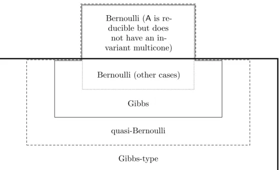
Figure 1 illustrates how different properties of equilibrium states for Φsare related. The following example shows that the inclusions depicted in the figure are strict.
Example 2.10. (1) It can happen that an equilibrium state for Φs is a Gibbs measure for some H¨older-continuous potential, but is not a Bernoulli measure: Choose two positive matrices
A1= 2 1
1 1
and A2 = 2 1
1 2
.
Then (A1, A2) is irreducible and has a strongly invariant multicone (i.e. the union of the first and third quadrants). The claim follows now from Theorem 2.9 and Proposition 2.7.
(2) It can happen that an equilibrium state for Φs is a quasi-Bernoulli measure, but is not a Gibbs measure for any H¨older-continuous potential: LetA1 andA2 be as above. Then (A1, A2, I)
Bernoulli (Ais re- ducible but does
not have an in- variant multicone) Bernoulli (other cases)
Gibbs quasi-Bernoulli
Gibbs-type
Figure 1. Classification of equilibrium states for Φs.
is irreducible and has an invariant multicone (i.e. the union of the first and third quadrants). The claim follows now from Theorems 2.8 and 2.9.
(3) It can happen that an equilibrium state for Φs is a Gibbs-type measure for Φs, but is not a quasi-Bernoulli measure: Choose two matrices
A3= 1 0
0 2
and A4 = 0 1
1 0
.
Then (A3, A4) is irreducible, has no invariant multicone, and does not contain only conformal matrices. The claim follows now from Proposition 2.6 and Theorem 2.8. We remark that this phenomenon has been observed earlier in [18,§1.4]. Another way to see the claim is to consider two conformal irreducible matrices not sharing a conjugation matrix.
3. Characterization of domination
In this section, we prove Theorem 2.1 and Propositions 2.2 and 2.3. LetA⊂GL2(R) and recall that S(A) is the sub-semigroup of GL2(R) generated by A. Let S(A) =RS(A)⊂M2(R) and note thatS(A) is a sub-semigroup of M2(R). Define
R(A) ={A∈S(A) : rank(A) = 1}.
Lemma 3.1. If A⊂GL2(R), then R(A) =∅ if and only if Ais strongly conformal.
Proof. IfAis strongly conformal, then by definition there exists a conjugation matrixM ∈GL2(R) such that|det(A)|−1/2M AM−1 ∈O(2) for all A∈A, which implies that |det(A)|−1/2M AM−1∈ O(2) for all nonzeroA∈S(A) =RS(A). In particular, all nonzero elements ofS(A) have rank 2 and thereforeR(A) =∅.
Suppose conversely thatR(A) =∅. We claim that set
S0(A) ={|det(A)|−1/2A:A∈S(A)\ {0}}=S(A)∩ {A∈M2(R) :|det(A)|= 1}
is compact. It is obviously closed, being the intersection ofS(A) with the closed set {A∈M2(R) :
|det(A)|= 1}. If it contains a sequence of elements (An) such that kAnk → ∞then this sequence can without loss of generality be taken to be a sequence of elements of RS(A). The sequence of normalised matriceskAnk−1An has an accumulation point which necessarily has determinant zero and norm one and belongs toS(A); this limit point is thus an element ofR(A), which is a
contradiction, and we conclude that{|det(A)|−1/2A:A∈S(A)\ {0}}is bounded. It is therefore compact as claimed.
The setS0(A) is thus a compact sub-semigroup ofGL2(R). We claim that it is a group. To show this it is sufficient to show that the inverse of everyA∈S(A) with|det(A)|= 1 belongs toS(A).
IfA∈S(A) is arbitrary, take a convergent subsequence (Ank)∞k=1 of the sequence (An)∞n=1 with limitB ∈S(A)⊂GL2(R), say. The sequence (A−nk)∞k=1 clearly converges toB−1 and therefore Ank+1−nk−1 →A−1 as k→ ∞. ThusA−1 is the accumulation point of a sequence of elements of S(A), hence an element of S(A).
The setS0(A) is therefore a compact subgroup ofGL2(R). Ifm is Haar measure onS0(A) and h·,·iis the standard inner product onR2 it is easy to see thathu, vi0 :=R
hAu, Avidm(A) defines an inner product on R2 which is invariant under every element of S0(A). Every inner product onR2 is related to the standard one by a change of basis, so there existsX ∈GL2(R) such that hu, vi0 =hXu, Xvi for all u, v∈R2. In particular, hXAX−1u, XAX−1vi =hAX−1u, AX−1vi0 = hX−1u, X−1vi0 =hu, vi for all u, v∈R2 and A∈S0(A) which yields S0(A)⊂XO(2)X−1. Thus S(A) is strongly conformal and thereforeA is strongly conformal as required.
We note that according to the previous lemma, R(A)6=∅ if and only if S(A) contains at least one proximal or parabolic element. In the next lemma, we exclude parabolic elements.
Lemma 3.2. Let A⊂GL2(R) with R(A) 6=∅ be such that S(A) is almost multiplicative. Then S(A) does not contain parabolic elements and R(A) does not contain nilpotent elements.
Proof. Suppose that S(A) contains a parabolic element. This means that, after a suitable change of basis, there existsA∈ S(A) such that
A= a 0
b a
,
where b 6= 0. It follows that there exists c > 0 such that c−1n|an−1b| 6 kAnk 6 cn|an−1b| for all n ∈ N. It follows directly that limn→∞kA2nk/kAnk2 = 0 which contradicts the condition kABk>κkAkkBk.
Observe that the relation kABk > κkAkkBk holds for all A, B ∈ S(A) by continuity. So similarly, if there exists a nilpotentA ∈R(A), then 0 =kAnk >κn−1kAkn >0 for some n∈N,
which is again a contradiction.
AssumingR(A)6=∅, we define the set Xu of all unstable directions of proximal elements ofS(A) to be
Xu =Xu(A) ={V ∈RP1:V =AR2 for someA∈R(A)}
and the setXs of allstable directions to be
Xs=Xs(A) ={ker(A)∈RP1:A∈R(A)}.
Lemma 3.3. LetA⊂GL2(R) with R(A)6=∅ be such that S(A) is almost multiplicative. Then the sets Xu andXs are nonempty, compact, and disjoint. Furthermore, AXu ⊂Xu for allA∈S(A).
Proof. First, we note again that the relationkABk>κkAkkBkholds for all A, B∈S(A). To see thatXu and Xs are disjoint, note that if V ∈Xu∩Xs then there exist nonzero B1, B2 ∈R(A) such thatB2R2 =V andB1V ={0}. HenceB1B2 is the zero matrix but B1 andB2 are not, which contradictskB1B2k>κkB1kkB2k>0. It follows that Xu∩Xs is empty. The nonempty set
R1(A) ={B ∈R(A) :kBk= 1}={B∈S(A) : det(B) = 0 andkBk= 1}
is clearly a closed bounded subset ofS(A), and in particular is compact. It follows thatXu and Xs are the images of continuous functions R1(A)→RP1 and hence are compact and nonempty.
To see the last claim, consider a subspaceU such that U =AV for someV ∈Xu andA∈S(A).
We have V = BR2 for some B ∈ R(A). Clearly AB has rank at most 1 and is nonzero since kABk>κkAkkBk>0, soAB∈R(A) and U ∈Xu.
The following lemma shows that the definitions of unstable and stable directions agree with the ones given in§2.1.
Lemma 3.4. Let A⊂GL2(R) withR(A)6=∅ be such thatS(A) is almost multiplicative. Then Xu ={u(A) :A∈ S(A) is proximal},
Xs={s(A) :A∈ S(A) is proximal}.
Proof. Let us first demonstrate the inclusions
Xu ⊂ {u(A) :A∈ S(A) is proximal}, (3.1) Xs⊂ {s(A) :A∈ S(A) is proximal}. (3.2) Before doing so, we show that for every A ∈R(A) with kAk = 1 and any sequence (Bn)∞n=1 of elements ofS(A) such that kBnk−1Bn →A as n→ ∞, the sequence Bn contains only proximal elements for all sufficiently large n. By Lemma 3.2, no Bn may be a parabolic matrix. Let us contrarily assume that, after passing to a suitable subsequence, every Bn is conformal. Write Bn0 :=kBnk−1Bnfor alln∈N. SinceAhas rank one we have det(A) = 0 and therefore det(B0n)→0.
Since everyBn0 is conformal it satisfies (trBn0)2 64|det(Bn0)|and therefore trBn0 →0. By the Cayley- Hamilton theorem, we have (Bn0)2−(trB0n)Bn0 + (det(Bn0))I =0 and sinceBn0 →A we deduce that (Bn0)2 → 0. Since kBn0k= 1 for all n∈Nwe get kBn2k/kBnk2 =k(Bn0)2k/kBn0k2 =k(B0n)2k →0, but this contradictskBn2k>κkBnk2. We conclude that (Bn)∞n=1 is proximal for all sufficiently large nas claimed.
It is well known that the mapsu(·) and s(·) are continuous on proximal matrices. Moreover, by Lemma 3.2, every A ∈ R(A) is proximal. Hence, if V ∈ Xu, then there exists a proximal A ∈ R(A) with kAk = 1 such that V = AR2 = u(A). Moreover, there exists a sequence of proximal matrices Bn ∈ S(A) such that kBnk−1Bn → A and thus, by the continuity of u, u(Bn) =u(kBnk−1Bn)→u(A) =V, which shows (3.1). Similarly, if V ∈Xs, then there exists a proximal A∈R(A) with kAk= 1 such that V = ker(A) =s(A), and there exists a sequence of proximal matricesBn∈ S(A) such thatkBnk−1Bn→A. Applying now the continuity of s, we get s(Bn) =s(kBnk−1Bn)→s(A) =V showing (3.2).
To finish the characterization ofXu it is sufficient to show that
Xu ⊃ {u(A) :A∈ S(A) is proximal}, (3.3) Xs ⊃ {s(A) :A∈ S(A) is proximal}, (3.4) since we may then appeal to Lemma 3.3 and the fact that the sets Xu and Xs are closed. If V =u(A) for some proximalA∈ S(A), then kAnk−1An→B asn→ ∞, where B ∈R(A) is such that BR2 = u(B) = V. This shows (3.3). Similarly, if V = s(A) for some proximal A ∈ S(A), thenkAnk−1An→B asn→ ∞, whereB ∈R(A) is such that ker(B) =V. This shows (3.4) and
completes the proof.
Letdbe the metric onRP1 defined by takingd(U, V) to be the angle between the subspaces U and V. IfA⊂GL2(R) is such that R(A)6=∅, then we define
Vn={U ∈RP1:d(U, V)< 1n for someV ∈Xu} and
Un= [
A∈S(A)
AVn
for all n∈N.
Lemma 3.5. Let A⊂GL2(R) with R(A) 6=∅ be such that S(A) is almost multiplicative. Then there is n0∈Nsuch that Un as defined above is an invariant unstable multicone for all n>n0.
Proof. Note that for all n∈Nthe invariance of Un and the property (2) in the definition of the unstable multicone (see§2.1) follow immediately from the definition of the setUnand the continuity of eachA∈ S(A) as an action onRP1. Let us prove the property (3) for alln∈N. ObviouslyVnis open, and since eachA∈ S(A) is invertible and therefore induces a homeomorphism of RP1, each Un is open too. It is clear from the definition that every connected component of Vn intersectsXu. IfU ∈ Un, thenU =AU0 for someA∈ S(A) andU0 ∈ Vn. Let I ⊂ Vn be an open connected set which containsU0 and which also intersects Xu. The set AI then contains U, is connected, and intersectsAXu. Since AXu⊂Xu by Lemma 3.3, we conclude that each connected component of Un intersectsXu.
To show that the property (1) holds for all large enoughn, let us suppose the contrary. In this caseUn∩Xs must be nonempty for infinitely many n∈N. This implies that in any prescribed neighbourhoods ofXu andXs we may find a subspaceU in the neighbourhood ofXu and a matrix A ∈ S(A) such that AU belongs to the neighbourhood of Xs. It follows that we may choose a sequence of subspaces (Un) converging to a limitU ∈Xu and a sequence (An) of elements ofS(A) such thatAnUnconverges to a limitV ∈Xs. DefineBn:=kAnk−1An∈S(A) for everyn∈N, and by passing to a subsequence if necessary we may suppose that (Bn) converges to a limitB ∈S(A) with norm 1.
We claim that BU = V. Let (un) be a sequence of unit vectors such that un ∈Un for every n∈ N and such that (un) converges to a unit vector u ∈ U. It is enough to show that (Bnun) converges toBuand thatBuis nonzero, since we have then shown that V = limn→∞BnUn=BU. To see that Buis nonzero we note thatu∈U ∈Xu andB ∈S(A) withB 6= 0, so if Bu= 0 then u∈kerB ∈Xs and we haveU ∈Xs∩Xu contradicting Lemma 3.3. On the other hand since
06kBnun−Buk6kBnun−Bnuk+kBnu−Buk6kun−uk+kBn−Bk →0
we haveBnun→Buasn→ ∞as required. But the equationBU =V is impossible sinceBU ∈Xu by Lemma 3.3 and thereforeV ∈Xs∩Xu, contradicting Lemma 3.3. We conclude thatUn∩Xs must be empty for all large enoughnand therefore property (1) holds for all nsufficiently large.
We are left to show thatUnis a multicone. To that end, it suffices to show that ∂Un contains only finitely many points. To see this suppose for a contradiction thatU ∈RP1 is an accumulation point of a sequence (Uk)∞k=1 of distinct elements of ∂Un. We will find it convenient to identify a small open neighbourhood I of U with a bounded open interval (a, b) ⊂ R. By passing to a subsequence if necessary we may assume that (Uk)∞k=1 is monotone with respect to the natural order onI, and without loss of generality we assume (Uk)∞k=1 to be strictly increasing.
We assert that every interval (Uk, Uk+2) contains a point ofXu. Since Uk+1 is in the closure of Un, there exists a point of Un in the interval (Uk, Uk+2). Since neither Uk nor Uk+2 can belong to Un, it follows that some connected component ofUn is contained wholly within the interval (Uk, Uk+2). By (3), this implies that a point ofXu must lie in the interval (Uk, Uk+2). Since this is true for everyk∈N, it follows that U is an accumulation point ofXu and hence, by Lemma 3.3,U belongs toXu. ButXu is a subset ofUnand therefore U ∈ Un, which implies that Uk∈ Un for all sufficiently large k. This is clearly impossible since no element of ∂Un can be an element of Un.
This contradiction proves that∂Un must be finite.
The above lemmas prove Theorem 2.1:
Proof of Theorem 2.1. If R(A) = ∅, then, by Lemma 3.1, the set A is strongly conformal. If R(A)6=∅, then the claim follows from Lemmas 3.2 and 3.5.
Let us next turn to the proof of the propositions.
Lemma 3.6. Let A∈GL2(R) and let C be a multicone such that AC ⊂ C. IfA is conformal, then AC=C.
Proof. By a suitable change of basis, we may assume that A ∈ O(2). In this case A, preserves Lebesgue measure onRP1. IfAC(C, then, sinceCis a finite union of closed projective intervals and Ais a homeomorphism,ACmust have smaller Lebesgue measure thanC, which is a contradiction.
We remark that the converse statement is false: ifA is proximal and C is a closed projective interval with one endpoint equal tou(A) and the other endpoint equal tos(A), thenAC=C butA is not conformal.
IfA⊂GL2(R) and Ae is the collection of all conformal elements ofA, then we write F(A) :=S({|det(A)|−1/2A:A∈Ae}).
Lemma 3.7. Let A ⊂GL2(R) be such that R(A) 6=∅ and Ae be the collection of all conformal elements of A. If C is an invariant unstable multicone of A, then Ae={A∈A:AC =C}is strongly conformal and F(A) is finite.
Proof. SinceAhas an invariant multiconeC, it follows from Lemma 3.6 that AC=C for allA∈Ae. HenceAe ⊂ {A∈A:AC=C}.
Write A0e = {|det(A)|−1/2A : A ∈ A and AC = C}. Let us first assume that #∂C > 2. Let B1, B2 ∈ S(A0e) and suppose that B1 and B2 induce the same permutation of∂C. Then B1−1B2
fixes every point of∂C and therefore has more than 2 invariant subspaces and is necessarily equal to±I. It follows that in this case S(A0e) has at most 2(#∂C)! distinct elements. Let us now assume that #∂C= 2. Write∂C={U1, U2}, and let u1 ∈U1 andu2∈U2 be so that {u1, u2} is a basis for R2. Every element of S(A0e) preserves ∂C and hence is either diagonal or antidiagonal in this basis (where by an antidiagonal matrix we mean a 2×2 matrix with both main diagonal entries equal to zero and both other entries nonzero). Let Dbe the matrix which Du1 =u1 and Du2 =−u2. A diagonal element ofS(A0e) cannot be proximal since then eitherU1 orU2 would be the stable space of that matrix contradicting the propertyXs∩ C=∅of the unstable multiconeC. It follows that every diagonal element ofS(A0e) must belong to {±I,±D}. Let A1, . . . , A` be the anti-diagonal elements of A0e and define S={±I,±D} ∪ {±A1, . . . ,±A`} ∪ {±DA1, . . . ,±DA`}. The setS is a semigroup sinceAiD=−DAi and since eachAiAj is diagonal and hence equal to ±I or±D. In particular,S(A0e) is contained in a finite semigroup. Thus,A0e is strongly conformal, which implies
that{A∈A:AC=C} ⊂Ae.
Lemma 3.8. Let A⊂GL2(R) be such thatAhas an invariant unstable multicone C and S(A) does not contain parabolic elements. Let Ae be the collection of all conformal elements of A. Then
A1F1· · ·AnFnC ⊂ Co
for alln>(#∂C)2+ 1, A1, . . . , An∈A\Ae, and F1, . . . , Fn∈ F(A).
Proof. It is sufficient to show that every point of ∂C is mapped into C◦ byA1F1· · ·AnFn. Clearly, if there exists`∈ {1, . . . , n} such thatA`F`· · ·AnFnC ⊂ Co, then our claim follows.
Suppose for a contradiction that there existn>(#∂C)2+1,A1, . . . , An∈A\Ae, andF1, . . . , Fn∈ F(A) such that for every `∈ {1, . . . , n} there exist V`, W`∈∂C for which
A`F`· · ·AnFnV`=W`.
Since n>(#∂C)2+ 1, there exist `1 < `2 such thatV`1 =V`2 and W`1 =W`2. Hence, A`1F`1· · ·A`2−1F`2−1W`2 =W`2.
Thus, ifA`1F`1· · ·A`2−1F`2−1 is proximal, thenW`2 ∈Xu∪Xs. This is impossible, since∂C ∩(Xs∪ Xu) = ∅.If A`1F`1· · ·A`2−1F`2−1 is conformal, then A`1F`1· · ·A`2−1F`2−1C = C by Lemma 3.6.
This is also impossible, sinceC)A`1C ⊃A`1F`1· · ·A`2−1F`2−1C by Lemma 3.7.
Lemma 3.9. Let A⊂GL2(R) be such thatAhas an invariant unstable multicone C and S(A) does not contain parabolic elements. LetAe be the collection of all conformal elements of A. IfA\Ae is compact, then
B={A1A2:A1∈A\Ae andA2∈ F(A)}
has a strongly invariant multicone.
Proof. Write m= (#∂C)2+ 1 and note that, by Lemma 3.8,Bm has a strongly invariant multicone.
SinceA\Ae is compact by the assumption andF(A) is finite by Lemma 3.7, Bm is compact. Hence, by [7, Theorem B], Bm is dominated, i.e. there exist constantsC >0 andτ >1 such that
kB1· · ·Bnk
k(B1· · ·Bn)−1k−1 >Cτn.
for allB1, . . . , Bn∈Bm and all n∈N. Choosek∈Nand let AiFi∈Bfor alli∈ {1, . . . , k}. Write k=qm+p, whereq ∈N∪ {0}and p∈ {0, . . . , m−1}. Then
kA1F1· · ·AkFkk
k(A1F1· · ·AkFk)−1k−1 = kB1· · ·Bq·Ak−pFk−p· · ·AkFkk k(B1· · ·Bq·Ak−pFk−p· · ·AkFk)−1k−1
> kB1· · ·Bqkk(Ak−pFk−p· · ·AkFk)−1k−1 k(B1· · ·Bq)−1k−1kAk−pFk−p· · ·AkFkk
>Cτqk(Ak−pFk−p· · ·AkFk)−1k−1 kAk−pFk−p· · ·AkFkk .
By choosing C0 = Cτ−1min`∈{1,...,m−1}k(A1F1· · ·A`F`)−1k−1/kA1F1· · ·A`F`k and τ0 =τ1/m, it follows again from [7, Theorem B] that Bhas a strongly invariant multicone.
The following lemma is [8, Lemma 2.2].
Lemma 3.10. Let C0,C ⊂ RP1 be multicones such that C0 ⊂ Co. Then there exists a constant κ0 >0 such that kA|Vk>κ0kAk for all V ∈ C0 and for every matrix A∈GL2(R) withAC ⊂ C0.
We are now ready to prove the propositions:
Proof of Proposition 2.2. The assertion (2) follows immediately from Lemma 3.7. Let us verify (1).
IfAe=A, thenS(A) is strongly conformal since Ais. This means that S(A) does not contain an proximal matrix and thus,Acannot have an unstable multicone by definition. Therefore, (1) holds.
To prove the final claim, it is sufficient to show that, by assumingA\Ae to be compact, there exists an invariant multiconeC such that AC ⊂ Co for all A∈A\Ae andAC=C for all A∈Ae. By Lemma 3.7, the setF(A) is finite. Therefore, the setB={A1A2:A1∈A\Ae and A2 ∈ F(A)}
is compact and, by Lemma 3.9, it has a strongly invariant multiconeC0. Defining C = [
F∈F(A)
FC0,
we have
AC= [
F∈F(A)
AFC0⊂ C0o ⊂ Co.
for all A∈A\Ae. We have finished the proof since for any A∈Ae,AC=C holds trivially.
Proof of Proposition 2.3. Let ε >0 and define C0 = [
F∈F(A)
F
U ∈RP1:d(U, V)6εfor someV ∈ [
A∈Ah
AC
Recall that F(A) is finite by Lemma 3.7. By compactness of Ah, we may choose ε > 0 small enough so that C0 ⊂ Co,AC ⊂ C0 for all A∈Ah, and AC0 =C0 for all A∈Ae. Observe that every elementA∈ S(Ah∪Ae) can be written in the form (c0c1· · ·ck)F0Qk
i=1AiFi, whereci ∈R\ {0}, k∈N∪ {0},Ai∈Ah, and Fi ∈ F(A). Therefore, AC ⊂ C0 for allA∈ S(Ah∪Ae)\ S(Ae).
By Lemma 3.10, there exists a constantκ0=κ0(C0,C) such thatkA|Vk>κ0kAk for all V ∈ C0 and for every matrixA∈GL2(R) withAC ⊂ C0. Hence,
kABk>kAB|Vk=kA|BVkkB|Vk>κ20kAkkBk.
for all A, B ∈ S(Ah ∪Ae)\ S(Ae). If A ∈ S(Ae) or B ∈ S(Ae), then kABk > κ0kAkkBk holds
trivially for some κ0 >0 by the finiteness ofF(A).
4. Classification of equilibrium states
This section is devoted to the proofs of Propositions 2.6 and 2.7, and Theorems 2.8 and 2.9. In order to keep the proof of Theorem 2.9 as readable as possible, we have postponed the proof of a key technical lemma, Lemma 4.6, into §5. Before we start with the proof of the propositions, we state a couple of auxiliary lemmas.
We recall that λu(A) is the eigenvalue of A with the largest absolute value, and similarly, λs(A) is the eigenvalue ofA with the smallest absolute value. Note that |λu(A)|=kA|u(A)k and
|λs(A)|=kA|s(A)k, where u(A) is the eigenspace corresponding to λu(A) ands(A) the eigenspace corresponding toλs(A).
The following two lemmas are special cases of the result of Protasov and Voynov; see [32, Theorem 2]. In order to keep the paper as self-contained as possible, we give here alternative proofs.
Lemma 4.1. LetA= (A1, . . . , AN)∈GL2(R)N be such that all the elements ofA are proximal.
Then the following two statements are equivalent:
(1) λu(AiAj) =λu(Ai)λu(Aj) for all i, j,
(2) u(Ai) =u(Aj) for all i, j or s(Ai) =s(Aj) for all i, j.
Proof. It is easy to see that (2) implies (1). Let us show that (1) implies (2). By the assumption and the multiplicativity of the determinant, we have λs(AiAj) =λs(Ai)λs(Aj) for all i, j. First note that s(Ai) 6= u(Aj), for any i 6= j. Indeed, s(Ai) = u(Aj) would imply that the matrix AiAj has eigenvalue λs(Ai)λu(Aj). Thus, eitherλs(Ai)λu(Aj) =λu(Ai)λu(Aj) or λs(Ai)λu(Aj) = λs(Ai)λs(Aj), which implies that either λs(Ai) =λu(Ai) orλu(Aj) =λs(Aj), which contradicts to the proximality.
We prove the statement by induction. Since s(A1)6=u(A2), after a suitable change of basis, the matricesA1 and A2 have the form
A1 =
λu(A1) 0 a λs(A1)
and A1 =
λu(A1) b 0 λs(A1)
.
Hence, tr(A1A2) =λu(A1A2) +λs(A1A2) =λu(A1)λu(A2) +λs(A1)λs(A2) +ab. Soab= 0, which implies that ifb= 0 then s(A1) =s(A2) or ifa= 0 thenu(A1) =u(A2).
Let us then assume that the firstN−1 matrices have the property that eitheru(Ai) =u(Aj) for alli, j∈ {1, . . . , N−1} or s(Ai) =s(Aj) for alli, j∈ {1, . . . , N−1}. We may assume without loss of generality thatu(Ai) = u(Aj) for all i, j∈ {1, . . . , N−1}. For a fixedi∈ {1, . . . , N−1}
the equation λu(Ai)λu(AN) = λu(AiAN) holds only if u(Ai) = u(AN) or s(Ai) = s(AN). If u(Ai) =u(AN) for somei∈ {1, . . . , N−1}, then the proof is complete; otherwises(Ai) =s(AN) must hold for alli∈ {1, . . . , N−1}, which again implies the claimed property.
Lemma 4.2. LetA= (A1, . . . , AN)∈GL2(R)N be such that all the elements ofA are proximal.
The following two statements are equivalent:
(1) |λu(AB)|=|λu(A)λu(B)|for all A, B∈ S(A),
(2) u(Ai) =u(Aj) for all i, j or s(Ai) =s(Aj) for all i, j.
Proof. It is again easy to see that (2) implies (1). Therefore, we assume that (1) holds. Let us first show that λu(AiAj) =λu(Ai)λu(Aj) orλu(AiA2j) =λu(Ai)λu(Aj)2 for everyi6=j. Suppose for a contradiction that there existi6=j such that
λu(AiAj) =−λu(Ai)λu(Aj) and λu(AiA2j) =−λu(Ai)λu(Aj)2.
Hence,λu(AiAj)λu(Aj) =−λu(Ai)λu(Aj)2 =λu(AiA2j) and, by Lemma 4.1 applied to the matrix pair (AiAj, Aj), we have u(AiAj) =u(Aj) or s(AiAj) =s(Aj). Assuming u(AiAj) =u(Aj), we have−λu(Ai)λu(Aj)2v(Aj) =AjA2jv(Aj) =λu(Aj)2Aiv(Aj), where v(Aj)∈u(Aj) is a unit vector.
But this is a contradiction since this would imply thatλu(Ai) = 0 or λs(Ai) =−λu(Ai). The case s(AiAj) =s(Aj) is similar.