Simplex Differential Evolution

Simplex Differential Evolution

Musrrat Ali

¹

, Millie Pant

¹

and Ajith Abraham

²

1 Department of Paper Technology, Indian Institute of Technology Roorkee, Saharanpur campus, Saharanpur -247001, India

2 Machine Intelligence Research Labs (MIR Labs), Scientific Network for Innovation and Research Excellence, P.O. Box 2259, Auburn, Washington-98071- 2259, USA

musrrat.iitr@gmail.com, millidma@gmail.com, ajith.abraham@ieee.org

Abstract: Differential evolution (DE) algorithms are commonly used metaheuristics for global optimization, but there has been very little research done on the generation of their initial population. The selection of the initial population in a population-based heuristic optimization method is important, since it affects the search for several iterations and often has an influence on the final solution. If no a priori information about the optima is available, the initial population is often selected randomly using pseudorandom numbers.

In this paper, we have investigated the effect of generating the initial population without using the conventional methods like computer generated random numbers or quasi random sequences. We have applied non linear simplex method in conjugation of pseudorandom numbers to generate initial population for DE. Proposed algorithm is named as NSDE (using non linear simplex method), is tested on a set of 20 benchmark problems with box constraints, taken from literature and the numerical results are compared with results obtained by traditional DE and opposition based DE (ODE). Numerical results show that the proposed scheme considered by us for generating the random numbers significantly improves the performance of DE in terms of convergence rate and average CPU time.

Keywords: Stochastic optimization, differential evolution, crossover, initial population, random numbers

1 Introduction

DE is comparatively a recent addition to class of population based search heuristics. Nevertheless, it has emerged as one of the techniques most favored by engineers for solving continuous optimization problems. DE [1, 2] has several attractive features. Besides being an exceptionally simple evolutionary strategy, it is significantly faster and robust for solving numerical optimization problems and is more likely to find the function’s true global optimum. Also, it is worth mentioning that DE has a compact structure with a small computer code and has

fewer control parameters in comparison to other evolutionary algorithms.

Originally Price and Storn proposed a single strategy for DE, which they later extended to ten different strategies [3].

DE has been successfully applied to a wide range of problems including Batch Fermentation Process [4], Optimal design of heat exchanges [5], synthesis and optimization of heat integrated distillation system [6], optimization of non-linear chemical process [7], optimization of process synthesis and design problems [8], optimization of thermal cracker operation [9], optimization of water pumping system [10], dynamic optimization of a continuous polymer reactor [11], optimization of low pressure chemical vapor deposition reactors [12], etc.

Despite having several striking features and successful applications to various fields DE is sometimes criticized for its slow convergence rate for computationally expensive functions. By varying the control parameters the convergence rate of DE may be increased but it should be noted that it do not affect the quality of solution. Generally, in population based search techniques like DE an acceptable trade-off should be maintained between convergence and type of solution, which even if not a global optimal solution should be satisfactory rather than converging to a suboptimal solution which may not even be a local solution. Several attempts have been made in this direction to fortify DE with suitable mechanisms to improve its performance. Most of the studies involve the tuning or controlling of the parameters of algorithm and improving the mutation, crossover and selection mechanism, some interesting modifications that helped in enhancing the performance of DE include introduction of greedy random strategy for selection of mutant vector [13], modifications in mutation and localization in acceptance rule [14], DE with preferential crossover [15], crossover based local search method for DE [16], self adaptive differential evolution algorithm [17], new donor schemes proposed for the mutation operation of DE [18], parent centric DE [28]. All the modified versions have shown that a slight change in the structure of DE can help in improving its performance. However, the role of the initial population, which is the topic of this paper, is widely ignored. Often, the whole area of research is set aside by a statement “generate an initial population,”

without implying how it should be done. There is only few literature is available on this topic [23-27]. An interesting method for generating the initial population was suggested by Rahnamayan et al ([19], [20]) in which the initial population was generated using opposition based rule. To further continue the research in this direction, in this paper we propose two modified versions of DE to improve its performance in terms of convergence rate without compromising with the quality of solution. The modified version presented in this paper is named non linear simplex method called NSDE. In the present study our aim is to investigate the effect of initial population on payoff between convergence rate and solution quality. Our motivation is to encourage discussions on methods of initial population construction. Performances of the proposed algorithms are compared with Basic DE and differential evolution initialized by opposition based learning

(ODE), which is a recently modified version of differential evolution [19], on a set of twenty unconstrained benchmark problems.

Remaining of the paper is organized in following manner; in Section 2, we give a brief description of DE. In Section 3, the proposed algorithms are explained.

Section 4 deals with experimental settings and parameter selection. Benchmark problems considered for the present study are given in Section 5. The performances of the proposed algorithms are compared with basic DE and ODE in Section 6. The conclusions based on the present study are finally drawn in Section 7.

2 Differential Evolution (DE)

DE starts with a population of NP candidate solutions which may be represented as Xi,G, i = 1, . . . ,NP, where i index denotes the population and G denotes the generation to which the population belongs. The working of DE depends on the manipulation and efficiency of three main operators; mutation, reproduction and selection which briefly described in this section.

Mutation: Mutation operator is the prime operator of DE and it is the implementation of this operation that makes DE different from other Evolutionary algorithms. The mutation operation of DE applies the vector differentials between the existing population members for determining both the degree and direction of perturbation applied to the individual subject of the mutation operation. The mutation process at each generation begins by randomly selecting three individuals in the population. The most often used mutation strategies implemented in the DE codes are listed below.

DE/rand/1: _{, ,}

* (

_{, ,}

)

3 2

1g r g r g

r g

i X F X X

V = + − (1a)

DE/rand/2: V_i,g=X_r1,g+F*(X_r2,g−X_r3,g)+F*(X_r4,g−X_r5,g)

(1b)

DE/best/1: V_i,g = X_best,g +F

* (

X_r1,g −X_r2,g

)

(1c) DE/best/2:V_i,g = X_best,g +F*(X_r1,g−X_r2,g)+F*(X_r3,g −X_r4,g) (1d) DE/rand-to-best/1:

) (

* ) (

*

_{, , , ,}

,

,g r₁ g best g r₂ g r₃ g r₄ g

i X F X X F X X

V = + − + − (1e)

Where, i = 1, . . . , NP, r1, r2, r3 ∈ {1, . . . , NP} are randomly selected and satisfy:

r1 ≠ r2 ≠ r3 ≠ i, F ∈ [0, 1], F is the control parameter proposed by Storn and Price [1].

Throughout the paper we shall refer to the strategy (1a) which is apparently the most commonly used version and shall refer to it as basic version.

Crossover: once the mutation phase is complete, the crossover process is activated. The perturbed individual, Vi,G+1 = (v1,i,G+1, . . . , vn,i,G+1), and the current population member, Xi,G = (x1,i,G, . . . , xn,i,G), are subject to the crossover operation, that finally generates the population of candidates, or “trial”

vectors,Ui,G+1 = (u1,i,G+1, . . . , un,i,G+1), as follows:

, . 1 , . 1

, .

j i G j r

j i G

j i G

v if rand C j k

u x otherwise

+ +

≤ ∨ =

= ⎨⎧

⎩ ⁽²⁾

Where, j = 1. . . n, k ∈ {1, . . . , n} is a random parameter’s index, chosen once for each i, and the crossover rate, Cr ∈ [0, 1], the other control parameter of DE, is set by the user.

Selection: The selection scheme of DE also differs from that of other EAs. The population for the next generation is selected from the individual in current population and its corresponding trial vector according to the following rule:

. 1 . 1 .

. 1

.

( ) ( )

i G i G i G

i G

i G

U if f U f X

X X otherwise

+ +

+

⎧ ≤

= ⎨ ⎩

⁽³⁾

Thus, each individual of the temporary (trial) population is compared with its counterpart in the current population. The one with the lower objective function value will survive from the tournament selection to the population of the next generation. As a result, all the individuals of the next generation are as good or better than their counterparts in the current generation. In DE trial vector is not compared against all the individuals in the current generation, but only against one individual, its counterpart, in the current generation. The pseudo code of algorithm is given here.

DE pseudo code:

Step 1: The first step is the random initialization of the parent population.

Randomly generate a population of (say) NP vectors, each of n dimensions: xi,j= xmin,j + rand(0, 1)(xmax,j-xmin,j), where xmin,j and xmax are lower and upper bounds for j^th component respectively, rand(0,1) is a uniform random number between 0 and 1.

Step 2: Calculate the objective function value f(Xi) for all Xi.

Step 3: Select three points from population and generate perturbed individual Vi

using equation (1a).

Step 4: Recombine the each target vector xi with perturbed individual generated in step 3 to generate a trial vector Ui using equation (2).

Step 5: Check whether each variable of the trial vector is within range. If yes, then go to step 6 else make it within range using ui,j =2* xmin,j - ui,j ,if ui,j

< xmin,j and ui,j =2* xmax,j - ui,j , if ui,j> xmax,j, and go to step 6.

Step 6: Calculate the objective function value for vector Ui.

Step 7: Choose better of the two (function value at target and trial point) using equation (3) for next generation.

Step 8: Check whether convergence criterion is met if yes then stop; otherwise go to step 3.

3 Proposed NSDE Algorithm

In this section we describe the proposed NSDE algorithm and discuss the effect of embedding the proposed scheme in basic DE (as given in Section 2) on two simple benchmark examples taken from literature.

3.1 Differential Evolution with Non linear Simplex Method (NSDE)

The NSDE uses nonlinear simplex method (NSM) developed by J. A. Nelder and R. Mead [22], in conjugation with uniform random number to construct the initial population. The procedure of NSDE is outlined as follows:

1 Generate a population set P of size NP uniformly as in step 1 of DE and set k=1.

2 Generate a point by NSM Method, which has the following main operations.

2.1 Select n+ 1 point from population P randomly and evaluate function at these points.

2.2 Calculate the centroid of these points excluding the worst point, say Xmax at which function is maximum.

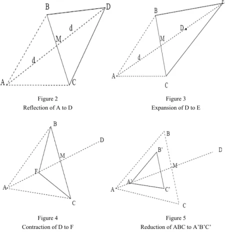
2.3 Reflection: Reflect Xmax through the centroid to a new point X1. And calculate the function value at this point.

2.4 Expansion: If f(X1)<=f(Xmin) then perform expansion to generate a new point X2 in the expanded region otherwise go to step 2.5. If f(X2)<f(Xmin) then include point X2 to the population Q otherwise point X1 is included to population Q and go to step 3.

2.5 Contraction: If f(X1)<f(Xmax) then produce a new point X3 by contraction otherwise go to step 2.6. If f(X3)<f(Xmax) then add point X3 to the population otherwise include point X1 to the population Q and go to step 3.

2.6 Reduction: Reduction is performed when either of the conditions mentioned above (from step 2.3 – step 2.5) are not satisfied. In this step we have replaced the original reduction method of Nelder Mead, by generating uniformly distributed random point say Xrand within the specified range and include it in the population Q and go to step 3.

3 If k<NP go to step 2.1 with k = k+1 else stop.

It can be seen from the above steps that in NSDE, initially a population set P of size NP is generated uniformly to which NSM is applied NP times to generate another population set Q so as to get a total population of size 2*NP. Finally, the initial population is constructed by selecting the NP fittest points from the union of P and Q. After initialization step, NSDE algorithm works like the basic DE.

With the use of NSM method, the initial population is provided with the information of the good regions that possess each particle as a vertex of the NSM simplex in each step. The algorithm is not computationally expensive, since for each particle of the initial population one function evaluation is done, which is inevitable even if we use a randomly distributed initial population.

Figure 2 Reflection of A to D

Figure 3 Expansion of D to E

Figure 4 Contraction of D to F

Figure 5 Reduction of ABC to A’B’C’

3.2 Effects of Using the Proposed NSDE to Generate Initial Population

The initial generation of population by nonlinear simplex method makes use of the function value to determine a candidate point for the additional population. As a result in the initial step itself we get a collection of fitter individuals which may help in increasing the efficiency of the algorithm. Consequently, the probability of obtaining the optimum in fewer NFEs increases considerably or in other words the convergence rate of the algorithm becomes faster. The initial generation of 100 points within the range [-2, 2] for Rosenbrock function and within the range [-600, 600] for Griewank function using basic DE, ODE and the proposed NSDE are depicted in Figs. 6(a)-6(c) and Figs. 7(a)-7(c) respectively. From these illustrations we can observe that the search space gets concentrated around the global optima which lies at (1, 1) with objective function value zero, for two dimensional Rosenbrock function and which lies at (0, 0) with objective function value 0, for Griewank function when the initial population is constructed using NSDE. The large search domain, [-600, 600], of Griewank function is contracted to the range of around [-400, 400] while using NSDE.

Figure 6 (a)

Initial population consisting of 100 points in the range [-2, 2] for Rosenbrock function using basic DE

Figure 6(b)

Initial population consisting of 100 points in the range [-2, 2] for Rosenbrock function using ODE

Figure 6 (c)

Initial population consisting of 100 points in the range [-2, 2] for Rosenbrock function using NSDE

Figure 7 (a)

Initial population consisting of 100 points in the range [-600, 600] for Griewanks function using DE

Figure 7 (b)

Initial population consisting of 100 points in the range [-600, 600] for Griewank function using ODE

Figure 7 (c)

Initial population consisting of 100 points in the range [-600, 600] for Griewank function using NSDE

4 Experimental Setup

With DE, the lower limit for population size, NP, is 4 since the mutation process requires at least three other chromosomes for each parent. While testing the algorithms, we began by using the optimized control settings of DE. Population size, NP can always be increased to help maintain population diversity. As a general rule, an effective NP is between 3 ∗ n and 5 ∗ n, but can often be modified depending on the complexity of the problem. For the present study we performed several experiments with the population size as well as with the crossover rate and mutation probability rate and observed that for problems up to dimension 30 a population size of 3*n is sufficient. But here we have taken fixed population size NP=100, which is slightly large than 3*n. Values of scale F, outside the range of 0.4 to 1.2 are rarely effective, so F=0.5 is usually a good initial choice. In general higher value of Cr help in speeding up the convergence rate therefore in the present study we have taken Cr =0.9. All the algorithms are executed on a PIV PC, using DEV C++, thirty times for each problem. In order to be fair we have kept the same parameter settings for all the algorithms. Random numbers are generated using the inbuilt random number generator rand ( ) function available in DEVC++.

Over all acceleration rate AR, which is taken for the purpose of comparison is defined as [19]

j j = 1

j 1

N F E ( b y o n e a l g o )

A R = 1 - 1 0 0

N F E ( b y o t h e r a l g o )

j μ

μ

=

⎛ ⎞

⎜ ⎟

⎜ ⎟ ×

⎜ ⎟

⎜ ⎟

⎝ ⎠

∑

∑

Where μ is number of functions. In every case, a run was terminated when the best function value obtained is less than a threshold for the given function or when the maximum number of function evaluation (NFE=10⁶) was reached. In order to have a fair comparison, these settings are kept the same for all algorithms over all benchmark functions during the simulations.

5 Benchmark Problems

The performance of proposed NSDE is evaluated on a test bed of twenty standard, benchmark problems with box constraints, taken from the literature [20].

Mathematical models of the benchmark problems along with the true optimum value are given in Appendix

.

6 Numerical Results and Comparisons

6.1 Performance Comparison of Proposed NSDE with Basic DE and ODE

We have compared the proposed algorithms with the basic DE and ODE. Here we would like to mention that we have used ODE version given in [19] instead of [20] because in [20], the authors have used the additional features like opposition based generation jumping, etc. while in the present study we just focusing on the effect of initial population generation on differential evolution algorithm.

Comparisons of the algorithms is done in terms of average fitness function value, standard deviation and the corresponding t-test value; average number of function evaluations and the average time taken by every algorithm to solve a particular problem. In every case, a run was terminated when the best function value obtained is less than a threshold for the given function [19] or when the maximum number of function evaluation (NFE=10⁶) was reached.

From Table 1, which gives the average fitness function value, standard deviation and t-values it can be observed that for the 20 benchmark problems taken in the present study all the algorithms gave more or less similar results in terms of average fitness function value, with marginal difference, which are comparable to true optimum. For the function f14 (Step function) all the algorithms gives same results. The best and worst fitness function values obtained, in 30 runs, by all the algorithms for benchmark problems are given in Table 3.

However when we do the comparison in terms of average time taken and average number of function evaluations then the proposed NSDE emerges as a clear

winner. It converges to the optimum at a faster rate in comparison to all other algorithms. Only for functions f13 (Schwefel) NSDE took more NFE than ODE, whereas for the remaining 19 problems NSDE converged faster than the basic DE and ODE. For solving 20 problems the average NFE taken by NSDE are 1334200 while ODE took 1794738 NFE and DE took 1962733 NFE. This implies that NSDE has an acceleration rate of around 35% in comparison to basic DE and an acceleration rate of 26% in comparison to ODE. ODE on the other hand reduces the NFE only up to 8.56%, in comparison to basic DE. A similar trend of performance can be observed from the average computational time. For solving 20 problems NSDE took least CPU time in comparison to the other two algorithms.

Performance curves of selected benchmark problems are illustrated in Figs. 8(a)- 8(h).

Table 1

Mean fitness, standard deviation of functions in 30 runs and t-valve Mean fitness, (Standard deviation) and t-value Function Dim.

DE ODE NSDE

f1 30 0.0546854

(0.0131867) --

0.0901626 (0.0077778)

12.48

0.0916686 (0.00721253)

13.25

f₂ 30 0.0560517

(0.0116127) --

0.0918435 (0.00565233)

14.92

0.0866163 (0.00666531)

12.29

f3 30 0.0957513

(0.00293408) --

0.0952397 (0.00499586)

0.48

0.0951172 (0.00405255)

0.68

f4 10 0.0931511

(0.0145175) --

0.0874112 (0.00699322)

1.92

0.0851945 (0.0121355)

2.26

f₅ 30 0.0915561

(0.012111) --

0.0885065 (0.00711877)

1.17

0.0916412 (0.00860403)

0.03

f6 30 0.0942648

(0.00478545) --

0.0933845 (0.00620528)

0.60

0.0926704 (0.00735851)

0.98

f7 2 4.26112e-008

(2.5783e-008) --

6.23824e-008 (2.75612e-008)

2.82

4.9999e-008 (2.95279e-008)

1.01

f₈ 4 0.0620131

(0.0239495) --

0.0528597 (0.0276657)

1.35

0.0591064 (0.0123711)

0.58

f9 30 0.088998

(0.00880246) --

0.092875 (0.00487147)

2.08

0.0882776 (0.0103789)

0.29

f₁₀ 10 -7.91444 (3.40729)

--

-9.61563 (0.024986)

2.69

-9.62952 (0.0238362)

2.71

f11 30 0.0842833

(0.00897659) --

0.0890837 (0.00961583)

1.97

0.0901177 (0.00969009)

2.38

f12 30 0.0940407

(0.00501821) --

0.0931232 (0.00502023)

0.69

0.0951981 (0.00373364)

0.99

f₁₃ 30 0.0956696

(0.00352899) --

0.0935369 (0.00397665)

2.16

0.0955274 (0.00495933)

0.13

f14 30 0.0

(0.0) --

0.0 (0.0)

--

0.0 (0.0)

--

f15 30 0.0730003

(0.0169434) --

0.0880257 (0.0115251)

3.95

0.0890936 (0.00986588)

4.42

f16 2 0.0645903

(0.0231492) --

0.0545825 (0.0263629)

1.54

0.0539806 (0.0226797)

1.76

f17 30 0.0910662

(0.00428958) --

0.0845474 (0.0118228)

2.79

0.0923214 (0.00514694)

1.01 f18 2 4.75455e-008

(2.9688e-008) --

3.63292e-008 (3.10335e-008)

1.41

2.657e-008 (2.657e-008)

1.49

f19 5 0.067335

(0.025448) --

0.0738969 (0.0209749)

1.07

0.0769911 (0.0160823)

1.73

f₂₀ 5 -3.99239

(0.00164918) --

-3.99398 (0.00235545)

2.98

-3.99297 (0.00184151)

1.27

Table 2

Average CPU time (in sec) taken by the algorithms, mean number of function evaluation of 30 runs and over all acceleration rates

Average Time (Sec) Mean function Fu

n. Dim.

DE ODE NSDE DE ODE NSDE f₁ 30 0.60 0.54 0.51 28020 26912 26220 f2 30 0.60 0.57 0.55 37312 36639 35500 f3 30 11.30 11.10 10.40 295232 295112 232860 f₄ 10 2.41 2.34 2.13 382454 361234 265420 f₅ 30 1.80 1.79 1.70 54503 53305 52240 f6 30 1.50 1.45 1.41 52476 51589 49170 f7 2 0.31 0.29 0.23 3845 3740 3520 f₈ 4 0.10 0.11 0.09 7902 7934 6780 f9 30 1.20 1.11 1.11 44034 41455 35330 f10 10 3.02 2.93 2.67 220356 196871 172200 f11 30 2.91 2.37 1.81 200924 196617 44960 f₁₂ 30 0.59 0.52 0.50 66154 63760 57800 f13 30 1.83 1.24 1.42 197069 148742 155970 f14 30 0.71 0.65 0.53 42423 41578 32300 f₁₅ 30 0.47 0.45 0.43 25903 24236 22620 f16 2 0.13 0.11 .10 3913 3832 3600 f17 30 0.92 0.81 0.76 55029 52455 47760 f18 2 0.23 .21 0.16 7367 7249 5150 f₁₉ 5 1.66 1.12 0.61 205398 150173 57540 f20 5 0.39 0.37 0.31 32419 31305 27260 Total 32.68 30.08 27.43 1962733 1794738 1434200

AR 7.955% 16.064% 8.5592 % 26.928 %

Table 3

Best and worst fitness function values obtained by all the algorithms Best and Worst function values Functi

on Dim.

DE ODE NSDE

f1 30 0.0533706 0.0920816

0.0710478 0.0980475

0.0801175 0.0989173 f2 30 0.0469366

0.0852506

0.0834493 0.0994759

0.0708503 0.0971761 f3 30 0.0912359

0.099449

0.0812952 0.0991723

0.085954 0.0987729 f₄ 10 0.0555946

0.0973456

0.0782872 0.0990834

0.0586798 0.0986525 f₅ 30 0.0550155

0.0985525

0.0765341 0.0976009

0.0730851 0.0988916 f6 30 0.0811647

0.0995538

0.0799383 0.0992613

0.0777488 0.0979521 f7 2 3.03242e-009

8.24678e-008

1.9059e-008 9.47894e-008

5.64424e-009 8.50966e-008 f8 4 0.0139037

0.0974824

0.00826573 0.0912189

0.0333435 0.0790444 f9 30 0.0746445

0.0995713

0.0849655 0.098311

0.064171 0.0992847 f₁₀ 10 -9.64801

-1.02642

-9.65114 -9.59249

-9.65368 -9.57805 f₁₁ 30 0.0627431

0.0944119

0.0636232 0.0989899

0.0683468 0.0994605 f12 30 0.0849009

0.0991914

0.0819181 0.0999306

0.0887407 0.0997806 f13 30 0.0902771

0.0996024

0.0866648 0.0988438

0.0854635 0.0998667

f14 30 0.0

0.0

0.0 0.0

0.0 0.0 f15 30 0.0441712

0.0945989

0.0593778 0.0991945

0.067818 0.0992816 f₁₆ 2 0.0277478

0.0969767

0.0129757 0.0984134

0.0297125 0.0918671 f₁₇ 30 0.0844465

0.0975161

0.0593988 0.0997203

0.0836182 0.0996487 f18 2 2.3063e-009

9.91416e-008

4.64862e-009 9.55725e-008

1.11418e-008 8.51751e-008 f19 5 0.00746793

0.099394

0.0291998 0.0995076

0.0483536 0.0999149 f20 5 -3.99626

-3.99019

-3.99737 -3.99035

-3.99644 -3.99027

0 20 40 60 80 100 120 140 160

500 5500 10500 15500

FItness

NO  of function evaluation DE ODE NSDE

0 10 20 30 40 50 60 70

500 1500 2500 3500 4500 5500 6500

Fitness

NO of function evaluation DE ODE NSDE

Figure 8(a) Sphere (f1) function

Figure 8(b) Colville (f8) function

0 2 4 6 8 10

20000 25000 30000 35000

Fitness

NO of function evaluation DE ODE NSDE

0 50 100 150 200 250 300 350 400 450

1000 6000 11000 16000 21000

Fitness

NO of function evaluation DE ODE NSDE

Figure 8(c) Axis parallel (f2) function

Figure 8(d) Griewenk (f5) function

0 10 20 30 40 50 60 70 80 90 100

500 50500 100500 150500 200500 250500

Fitness

NO of function evaluation DE ODE NSDE

‐4.5

‐4

‐3.5

‐3

‐2.5

‐2

‐1.5

500 5500 10500 15500 20500 25500

Fitness

NO of function evaluation

DE ODE NSDE

Figure 8(e) Restrigin (f4) function

Figure 8(f) Inverted (f20) cosine

0 0.5 1 1.5 2 2.5 3 3.5 4 4.5

500 1000 1500 2000 2500 3000 3500

Fitness

NO of function evaluation DE ODE NSDE

0 1 2 3 4 5 6

500 3500 6500 9500 12500

Fitnessx 10000

NO of function evaluation DE ODE NSDE

Figure 8(g) Tripod (f16) function

Figure 8(h) Step (f14) function

Figures 8(a)-8(h)

Performance curves of few elected benchmark problems

Figure 9

Average number of function evaluations taken by DE, ODE and NSDE for the 20 benchmark problems

Figure 10

Average CPU time (in sec) taken by DE, ODE and NSDE for the 20 benchmark problems

Discussion and Conclusions

In the present paper we have proposed a simple and modified variant of DE namely NSDE. The only structural difference between the proposed NSDE and the basic DE lies is the generation of initial population. NSDE applies nonlinear simplex method to generate the initial population. From the empirical studies and graphic illustrations we can say that the proposed schemes enhance the working of basic DE in terms of average CPU time and NFEs without compromising with the quality of solution. Also we would like to mention that other than the process of initial population construction, we have not made use of any other additional feature/parameter in the basic structure of DE. Though we have applied the proposed schemes in basic DE, they can be applied in any evolutionary algorithm which makes use of randomly generated initial points. As a concluding statement it can be said that providing the initial population with some extra information of search space is an important help for the DE algorithm, since it may lead to faster convergence and better quality of the solutions provided by the algorithm.

References

[1] R. Storn, K. Price, “DE-a Simple and Efficient Adaptive Scheme for Global Optimization over Continuous Space”, Technical Report TR-95-012, ICSI, March 1995. Available via the Internet: ftp.icsi.berkeley.edu/pub/

techreports/ 1995/tr-95-012.ps.Z, 1995

[2] R. Storn, K. Price, “DE-a Simple and Efficient Heuristic for Global Optimization over Continuous Space”, Journal of Global Optimization 11(4), 1997, pp. 41-359

[3] K. Price, “An Introduction to DE”, In: Corne, D., Marco, D., Glover, F.

(eds.), New Ideas in Optimization, McGraw-Hill, London (UK), 1999, pp.

78-108

[4] F. S. Wang, W. M. Cheng, “Simultaneous Optimization of Feeding Rate and Operation Parameters for Fed-Batch Fermentation Processes”, Biotechnology Progress 15, 1999, pp. 949-952

[5] B. V. Babu, S. A. Munawar, “Differential Evolution for the Optimal Design of Heat Exchangers”, In: Proceedings of All-India seminar on Chemical Engineering Progress on Resource Development: A Vision 2010 and Beyond, Bhuvaneshwar, 2000

[6] B. V. Babu, R. P.Singh, “Synthesis & Optimization of Heat Integrated Distillation Systems Using Differential Evolution”, In: Proceedings of All- India seminar on Chemical Engineering Progress on Resource Development: A Vision 2010 and Beyond, Bhuvaneshwar, 2000

[7] R Angira, B. V. Babu, “Optimization of Non-Linear Chemical Processes Using Modified Differential Evolution (MDE)”, In: Proceedings of the 2^nd Indian International Conference on Artificial Intelligence, Pune, India, 2005a, pp. 911-923

[8] R. Angira, B. V. Babu, “Optimization of Process Synthesis and Design Problems: A Modified Differential Evolution Approach”, Chemical Engineering Science 61, 2006a, pp. 4707-4721

[9] B. V. Babu, R. Angira, “Optimization of Thermal Cracker Operation using Differential Evolution”, In: Proceedings of International Symposium & 54^th Annual Session of IIChE, Chennai, 2001b

[10] B. V. Babu, R. Angira, “Optimization of Water Pumping System Using Differential Evolution Strategies”, In: Proceedings of The Second International Conference on Computational Intelligence, Robotics, and Autonomous Systems, Singapore, 2003

[11] M. H. Lee, C. Han, K. S. Chang, “Dynamic Optimization of a Continuous Polymer Reactor Using a Modified Differential Evolution Algorithm”, Industrial and Engineering Chemistry Research 38, 1999, pp. 4825-4831 [12] J. C. Lu, F. S. Wang, “Optimization of Low Pressure Chemical Vapor

Deposition Reactors Using Hybrid Differential Evolution”, Canadian Journal of Chemical Engineering 79, 2001, pp. 246-254

[13] P. K Bergey, C. Rgsdale, “Modified Differential Evolution: a Greedy Random Strategy for Genetic Recombination”, omega 33, 2005, pp. 255- 265

[14] P. Kaleo, M. M. Ali, “A Numerical Study of Some Modified Differential Evolution Algorithms”, European journal of operational research 169, 2006, pp. 1176-1184

[15] M. M. Ali, “Differential Evolution with Preferential Crossover”, European Journal of Operational Research 181, 2007, pp. 1137-1147

[16] N. Noman, H. Iba, “Enhancing Differential Evolution Performance with Local Search for High Dimensional Function Optimization”, GECCO’05 Washington, DC, USA, 2005, pp. 967-974

[17] A. K. Qin, P. N. Suganthan, “Self Adaptive Differential Evolution Algorithm for Numerical Optimization”, IEEE, 2005, pp. 1785-1791

[18] H. Y. Fan, J. Lampinen, G. S. Dulikravich, “Improvements to Mutation Donor Formulation of Differential Evolution”, International Congress on Evolutionary Methods for Design, Optimization and Control with Applications to Industrial Problems, EUROGEN, 2003, pp. 1-12

[19] Shahryar Rahnamayan, H. R. Tizhoosh, M. M. A. Salama, “A Novel Population Initialization Method for Accelerating Evolutionary Algorithms”, computer and applied mathematics with application 53, 2007, pp. 1605-1614

[20] S. Rahnamayan, H. R. Tizhoosh, M. A Salman, “Opposition-based Differential Evolution”, IEEE transaction on evolutionary computation 12(1), 2008, pp. 64-79

[21] M. M. Ali, A. Torn, “Population Set-based Global Optimization Algorithms: Some Modifications and Numerical Studies”, www.ima.umn.edu/preprints/, 2003

[22] J. A. Nelder, R mead, “A Simplex Method for Function Minimization”, computer journal, Vol. 7, 1965, pp. 308-313

[23] S. Kimura, K. Matsumura, “Genetic Algorithms using low discrepancy sequences”, in proc. of GEECO 2005, pp. 1341-1346

[24] Nguyen X. H., Nguyen Q. Uy., R. I. Mckay, P. M. Tuan, “Initializing PSO with Randomized Low-Discrepancy Sequences: The Comparative Results”, In Proc. of IEEE Congress on Evolutionary Algorithms, 2007, pp. 1985- 1992

[25] S. Kimura, K. Matsumura, “Genetic Algorithms Using Low Discrepancy Sequences”, in proceedings of the GECCO, 2005, pp. 1341-1346

[26] KE Parsopoulos, MN Vrahatis, “Initializing the Particle Swarm Optimization Using Nonlinear Simplex Method”, in advances in intelligent systems, fuzzy systems, evolutionary computation, WSEAS press, 216-221, 2002

[27] Millie Pant, Radha Thangaraj, Crina Grosan, Ajith Abraham “Improved Particle Swarm Optimization with Low-Discrepancy Sequences”, In Proc.

of IEEE Congress on Evolutionary Algorithms, 2008, pp.

[28] Millie Pant, Musrrat Ali, V. P. Singh “Differential Evolution with Parent Centric Crossover”, In Proc. of IEEE Congress on Evolutionary Algorithms, 2008, pp. 141-146

Appendix

1 Sphere function:

( )

²

1

1 n

i i

f x x

=

=

∑

^{, With}

^{− 5.12 ≤ ≤ x}

ⁱ

^5.12

^{, min} f1

( 0,..., 0 )

=

0

2 Axis parallel hyper-ellipsoid:

( )

²

2

1 n

i i

f x ix

=

=

∑

^{, with}

^{− 5.12 ≤ ≤ x}

ⁱ

^5.12

^{, min f2}

^{( 0,..., 0 )}

⁼

⁰

3 Rosenbrock’s valley:

( )

^{1 2 2 2}

3 1

1

[100( ) (1 )]

n

i i i

i

f x x x x

−

+

=

=

∑

− + − ^With

^{− ≤ ≤ 2 x}

ⁱ

²

^{, min f3}

^{( 1,...,1 )}

⁼

⁰

4 Restrigin’s function:

( )

²

4

1

10

ⁿ

(

_i

10 cos(2

_i

))

i

f x n x

π

x

=

= +

∑

− ^With

^{− 5.12 ≤ ≤ x}

ⁱ

^5.12

^{, min}

( )

4

0,..., 0 0

f =

5 Griewenk function:

( )

²

5

1 1

1 cos( ) 1

4000

n n

i i

i i

f x x x

i

= =

=

∑

−

∏

+ ^With

^{− 600 ≤ ≤ x}

ⁱ

⁶⁰⁰

^{, min}

( )

5

0,..., 0 0

f =

6 Ackley’s function:

6 ⁿ i^{2 n}

(

i

)

i 1 i 1

( ) 20*exp .2 1/n x exp 1/n cos 2 x 20

f X

π

e

= =

⎛ ⎞ ⎛ ⎞

= − ⎜⎜⎝−

∑

⎟⎟⎠− ⎜⎝

∑

⎟⎠+ + ^, With

− ≤ ≤ 32 x

_i

32

, min f6

( 0,..., 0 )

=

0

7 Beale function:

( )

^{2 2 2 3 2}

7 [1.5 1(1 2)] +[2.25 1(1 2)] +[2.625 1(1 2)]

f x = −x −x −x −x −x −x

With

− 4.5 ≤ ≤ x

_i

4.5

, min f7

( 3, 0.5 )

=

0

8 Colville function:

( )

^{2 2 2 2 2 2 2 2}

8 2 1 1 4 3 3 2 4

2 4

100( ) (1 ) 90( ) (1 ) 10.1(( 1) ( 1) )

19.8( 1)( 1)

f x x x x x x x x x

x x

= − + − + − + − + − + −

− −

,With

− ≤ ≤ 10 x

_i

10

, min f8

( 1,1,1,1 )

=

0

9 Levy function:

( )

^{2 1 2 2}

9 1 1

1

sin (3 ) ( 1)(1 sin (3 )) ( 1)(1 sin (2 ))

n

i i n n

i

f x

π

x ⁻ x

π

x₊ x

π

x

=

= +

∑

− + + − +

With

− ≤ ≤ 10 x

_i

10

, min f9

( 1,...,1 )

=

0

10 Michalewicz function:

( )

^{2 2}

10

1

sin( )(sin( ))

n

m

i i

i

f x x ix

π

=

= −

∑

^With

^{0 ≤ ≤ x}

ⁱ

^π

, m=10, min

10(_n 10)

9.66015

f ₌ = −

11 Zakharov function:

( )

^{2 2 4}

11

1 1 1

( 0.5 ) ( 0.5 )

n n n

i i i

i i i

f x x ix ix

= = =

=

∑

+

∑

+

∑

^With

^{− ≤ ≤ 5 x}

ⁱ

¹⁰

^{, min}

( )

11

0,..., 0 0

f =

12 Schawefel’s problem 2.22:

( )

12

1 1

n n

i i

i i

f x x x

= =

=

∑

+

∏

^With

^{− ≤ ≤ 10 x}

ⁱ

¹⁰

^{, min f12}

^{( 0,..., 0 )}

⁼

⁰

13 Schwefel’s problem 2.21:

( ) { }

13

max

_{i i}

,1

f x = x ≤ ≤i n With

− 100 ≤ ≤ x

_i

100

, min f13

( 0,..., 0 )

=

0

14 Step function:

( )

²

14

1

( 0.5 )

n i i

f x x

=

=

∑

⎢⎣ + ⎥⎦ ^With

^{− 100 ≤ ≤ x}

ⁱ

¹⁰⁰

^{, min}

( )

14 0.5 _i 0.5 0

f − ≤ ≤x =

15 Quartic function:

( )

⁴

[ )

15

1

0,1

n i i

f x ix random

=

=

∑

+ ^With

^{− 1.28 ≤ ≤ x}

ⁱ

^1.28

^{, min}

( )

15

0,..., 0 0

f =

16 Tripod function:

16

( ) ( )(1

2

( )) (

1 1

50 ( )(1 2 ( )))

2 1

(

2

50(1 2 ( )))

2

f x = p x +p x + x + p x − p x + x + − p x With

− 100 ≤ ≤ x

_i

100

, min

( )

16

0, 50 0 where ( ) 1 for 0 otherwise ( ) 0

f − = p x = x> p x =

17 Alpine function:

( )

17

1

sin( ) 0.1

n

i i i

i

f x x x x

=

=

∑

+ ^With

^{− ≤ ≤ 10 x}

ⁱ

¹⁰

^{, min f17}

^{( 0,..., 0 )}

⁼

⁰

18 Cshaffer’s function 6:

( )

^{2 12 22}

18 2 2 2

1 2

sin ( ) 0.5

0.5 1 0.01( )

x x

f x

x x

+ −

= +

+ + ^With

− ≤ ≤ 10 x

_i

10

, min

( )

18

0,0 0

f =

19 Pathological function:

( )

^{1 2 2 21}

19 2 2 2

1 1 1

sin (100 ) 0.5

0.5 1 0.001( 2 )

n

i i

i i i i i

x x f x

x x x x

− +

= + +

⎛ + − ⎞

⎜ ⎟

= +

⎜ + + − ⎟

⎝ ⎠

∑

With

− 100 ≤ ≤ x

_i

100

, min f19

( 0,..., 0 )

=

0

20 Inverted cosine wave function:

( )

^{1 2 21 1 2 2}

20 1 1

1

( 0.5 )

exp( ) cos(4 0.5 )

8

n

i i i i

i i i i

i

x x x x

f x x x x x

− + +

+ +

=

⎛ − + + ⎞

= − ⎜ + + ⎟

⎝ ⎠

∑

With

− ≤ ≤ 5 x

_i

5

, min f20

( 0,..., 0 )

= − +n

1