The probabilistic customer’s choice rule with a threshold attraction value: effect on the location of competitive facilities in the plane

The probabilistic customer’s choice rule with a threshold attraction value: effect on the location of

competitive facilities in the plane

Jos´e Fern´andez^∗

Dpt. of Statistics and Operations Research, University of Murcia, Murcia, Spain

Bogl´arka G.- T´oth

Institute of Informatics, University of Szeged, Szeged, Hungary

Juana L. Redondo and Pilar M. Ortigosa

Dpt. of Informatics, University of Almer´ıa, ceiA3, Almer´ıa, Spain

Abstract

The classical probabilistic choice rule assumes that customers patronize all the existing facilities. As this assumption may not be appropriate in some cases, in this paper a variant is investigated, in which a customer only pa- tronizes those facilities for which he/she feels an attraction greater than or equal to a threshold value. Implicitly, this implies that there may be some unmet demand. We apply this modified rule to the problem of locating a sin- gle new facility in the plane. A comparison of the location decisions derived from the modified rule with those obtained with the classical proportional choice rule when solving the location model reveals that the profit that the locating chain may lose if an inadequate choice rule is employed may be quite high in some instances.

Keywords:

Patronizing behavior, Customer choice rule, Competition, Continuous

∗Corresponding author

Email addresses: josefdez@um.es(Jos´e Fern´andez), boglarka@inf.u-szeged.hu (Bogl´arka G.- T´oth),{jlredondo, ortigosa}@ual.es(Juana L. Redondo and Pilar M.

Ortigosa)

URL: http://www.um.es/geloca/gio/josemain.html(Jos´e Fern´andez)

Location, Interval branch-and-bound method, Evolutionary algorithm, Computational study

1. Introduction

The patronizing behavior of customers is one of the core inputs in many business and economic indicators. This is the case for the estimation of the market share captured by the facilities in a competitive environment. When there exist several facilities offering the same product, the way in which customers decide to spend their buying power among them may determine the success or the failure of the facilities. Consumer behavior is a function of the attraction that consumers feel for the facilities. This attraction is the result of several factors, but the two most important forces are the location of the facilities and their quality.

Deciding the location and the quality of the new facilities to be opened is a hard task. There are many competitive location models in literature for that purpose. See for instance Eiselt and Laporte (1996), Eiselt et al. (1993), Plastria (2001) and the references therein. Depending on the location space, the number of facilities to be located, the type of competition, the demand and the way the attraction is measured, different location models have been proposed. Recently, in some of them, the quality of the new facility is also included as a variable to be determined (see Aboolian et al. (2007), Drezner et al. (2012), Fern´andez et al. (2007), Redondo et al. (2012, 2009b), Saidani et al. (2012)).

Of course, the patronizing behavior of customers is also taken into ac- count in location models, and this is the topic this paper is devoted to. Two choice rules are usually employed in literature. In the deterministic rule consumers are assumed to patronize only one facility, the one for which cus- tomers feel more attraction. However, this hypothesis has not found much empirical support, except in areas where shopping opportunities are limited and transportation is difficult. On the contrary, in the probabilistic rule, consumers patronize all the existing facilities, although the amount spent at each of them is different, and depends on the attraction of the consumers towards the particular facility. In general, this second rule has proved to ap- proximate the market share captured by the facilities more accurately than other alternatives.

However, does a customer really go to all the available facilities offering the product to satisfy his/her needs? To what extent does this assumption

have an influence on the selection of the location and the quality of the new facilities to be located? This is the research question studied in this paper. If the attraction that a demand point feels towards a facility is strictly positive, then, no matter how small that attraction is, according to the probabilistic rule the facility will capture part of the demand of the demand point. This may be unrealistic in some cases.

The idea of patronizing only some of the existing facilities is not new.

For example, in marketing literature, some theories of consumer behavior involve thresholds or discontinuities. For instance, in Gilbride and Allenby (2004) the authors investigate consumers’ use of screening rules as part of a discrete-choice model and they present a model that accommodates conjunc- tive, disjunctive, and compensatory screening rules. However, in the location literature this topic has been hardly investigated. We are only aware of three location papers. In the first one, the so-called Pareto-Huff rule (see Peeters and Plastria (1992)) was introduced. According to it, a customer patronizes a more distant facility only if that facility has a higher quality. The second paper Su´arez-Vega et al. (2007) introduces another variant, in which cus- tomers only patronize a facility provided that it offers a minimum attraction to them. Both papers deal withnetwork location problems. The third paper is Ghosh and Craig (1991), where the related concept of reservation distance is used in adiscretelocation model. In all the three papers it is assumed that the quality of the new facilities to be located are fixed and given beforehand.

In this paper we follow the idea in Su´arez-Vega et al. (2007), i.e., cus- tomers at each demand point have associated a minimum level of attraction in order to patronize a facility, and then they share their buying power among the facilities that pass this threshold. However, this paper differs from Ghosh and Craig (1991), Peeters and Plastria (1992) and Su´arez-Vega et al. (2007) in two key points: (i) we analyze location problems in the plane, and (ii) the quality of the new facilities is not given beforehand, but it is considered to be an additional variable of the problem to be determined. Both things make the problem much more challenging from the optimization point of view. It also differs from Peeters and Plastria (1992) and Su´arez-Vega et al. (2007) in two additional points: (iii) the function of the distance used in the attraction function does not have to be necessarily concave, and (iv) the locating chain does not have to be a new entrant in the market, it may already own some of the existing facilities. The variant of the probabilistic rule used in this pa- per, which will be referred to aspartially probabilistic choice rulehereinafter, is in many cases a more realistic assumption than that of the probabilistic

rule. Notice that when the attraction threshold is very low, this rule is sim- ilar to the proportional one. For higher threshold values this procedure may coincide with the deterministic rule. For intermediate threshold values, the customers’ choices may be different from both cases.

The use of attraction thresholds is related to the constrained choice-set concept used in Thill (2000) for the analysis of non-cooperative competition between multi-branch networks when consumers have heterogeneous prefer- ences. The implications of thresholds has also been investigated in some discrete choice models studies from different perspectives, considering them as minimum perceptible changes in attributes required for a decision maker (DM) to differentiate among alternatives (see for example Cantillo et al.

(2010, 2006), Cantillo and Ort´uzar (2006)). Those studies reveal that where perception thresholds exist in the population, the use of models without them leads to errors in estimation and prediction. However, in those papers the purpose is to analyze how the thresholds affect the decisions made by DMs, whereas in this paper we assume that perception thresholds exist in the cus- tomers and want to investigate its final influence in the location of the new facility.

In the location literature the use of thresholds is usually related to the distance. For example, in the location of some emergency facilities, the emer- gency facility is assumed not to provide a good response to a demand point if it is at a distance greater than a given threshold (see for instance Holmes et al. (1972) or Li et al. (2011)). In the location of some undesirable facilities, the undesirable effects produced by the facility are supposed to be negligible for a demand point if the facility is further than a given threshold distance (see for instance Plastria and Carrizosa (1999) or Yapicioglu et al. (2007)).

In covering location problems, a demand point is assumed to be covered by a facility if their interdistance is less than a given threshold (see Berman et al. (2010) and references therein). There are also competitive location papers where thresholds are used. For instance, there are location models in which the facilities to be located are required to capture a minimum level of demand (see for instance Colom´e et al. (2003)). When the deterministic choice rule is used, the location of the competitive facilities is fixed, and only the location is to be determined, then profit changes only occur at partic- ular threshold qualities (see Plastria and Carrizosa (2004)). There are also competitive location models where two facilities with the same quality are regarded as similar for a customer if the difference between the distances from the customer to the facilities is less than a given threshold (see Kress

and Pesch (2012) for a survey of that type of models on networks). The requirement of minimum level of attraction is also suggested in Arenoe et al.

(2015) (apart from Thill (2000) and Su´arez-Vega et al. (2007)).

Notice that if for a given demand point none of the facilities attains the minimum attraction level, then the demand at that demand point will not be served. Hence, in our model, it may exist some unmet demand. This feature also makes our model different from most of the models in the literature, where it is usually assumed that the whole demand is fully served. The most remarkable exceptions are the papers by Drezner and Drezner (2008, 2012), where the authors try to model the lost demand in a competitive environment similar to the one used in our paper (the probabilistic choice rule is explicitly considered in those two papers). However, the way in which lost demand is considered in those papers is different from the way it is done in our model.

In those papers, (i) all customers are partially served (part of their demand is not served) and (ii) the demand actually served at any given demand point is served from all the existing facilities. Furthermore, (iii) in Drezner and Drezner (2008) an exponential distance decay function is assumed to model the disutility of the facility as the distance between the demand point and the facility increases. On the contrary, in our model (i) some customers are fully served, whereas others may be not served at all, (ii) the demand at a given demand point may be served by only some of the existing facilities (not necessarily all) and the facilities which serve a demand point depend on the demand point, and (iii) a general distance decay function can be used in our model (in the computational studies we use a particular one, namely, a power of the distance, but other types of distance decay functions could be used as well, and the algorithms proposed in this paper can also handle them).

As we will see, the partially probabilistic choice rule can be modeled in continuous location problems without major difficulties. And even though the resulting problems are usually hard-to-solve global optimization problems (perhaps one of the reasons for which this choice rule has not been used before in continuous problems), they can be handled with the techniques presented in this paper. The aim of this paper is to study whether the location and quality of the new facilities to be located suggested by the location models differ depending on the choice rule employed.

The paper is organized as follows. The classical probabilistic choice rule is reviewed in the next section in the context of a continuous competitive facility location and design model. The partially probabilistic choice rule is

then introduced in the next section. Different approaches to solve the corre- sponding location problem are presented in Section 4. Some implementation issues related to the estimation of the parameters of the model are discussed in Section 5. The study of the influence of a particular customer choice rule in the decision about the optimal location and quality of a new facility is given in Section 6, whereas Section 7 shows a sensitivity analysis of the model to some of its parameters. Section 8 reports some computational studies to in- vestigate the effectiveness and efficiency of the methods proposed. The paper ends with Section 9 offering some conclusions and pointing lines for future research.

2. The probabilistic choice rule

A demand point aggregates the demand of all the consumers that it rep- resents. The probabilistic choice rule assumes that the demand at a demand point (or the buying power concentrated at it) is split probabilistically over all the facilities in the market proportionally to his/her attraction to each facility. Alternatively, it can be interpreted that customers patronize all the existing facilities (not just the most attractive to them), but the amount spent at each facility is proportional to the attraction that the customers feel towards the facility. This is the interpretation used throughout this paper, as well as in most of the location papers in the literature.

We will assume the following particular scenario (see Fern´andez et al.

(2007) for more details). A single new facility is going to be located in a given region of the plane by a chain. There already exist other facilities around selling the same goods or product. Some of those facilities may belong to the locating chain. The demand to be served, known and fixed, is concentrated at some demand points, whose locations are known. The location and quality of the existing facilities are also known. The attraction function of a demand point towards a facility is modeled as perceived quality divided by perceived distance.

The maximization of the profit obtained by the chain after the location of the new facility is the objective to be achieved, to be understood as the income due to the market share captured by the chain minus its operational costs. The aim is to find both the location and the quality of the new facility to be located.

The following notation will be used in the mathematical formulation of the location models:

Indices

i index of demand points, i= 1, . . . , i_max.

j index of existing facilities, j = 1, . . . , j_max (we assume that the first k of those j_max facilities belong to the locating chain (0≤k < j_max).

Variables

x location of the new facility,x= (x₁, x₂).

α quality of the new facility.

Data

p_i location of demand point i.

w_i demand (or buying power) concentrated at p_i. fj location of existing facilityj.

d_ij distance between demand pointp_i and facility f_j. α_j quality of facility f_j.

gi(·) a non-negative non-decreasing function.

u_ij attraction that p_i feels forf_j. In this paper, u_ij =α_j/g_i(d_ij).

d^min_i minimum distance fromp_i at which the new facility can be located.

α_min minimum level of quality.

α_max maximum level of quality.

S region of the plane where the new facility can be located.

G^ex fixed costs due to the existing chain-owned facilities.

Miscellaneous

d_i(x) distance between demand pointp_i and the new facility.

ui0(x, α) attraction that pi feels for the new facility; ui0(x, α)

=α/g_i(d_i(x)).

When a probabilistic rule is used, the market share captured by the chain is given by

M_P(x, α) =

imax

X

i=1

w_iu_i0(x, α) +Pk j=1u_ij u_i0(x, α) +Pjmax

j=1 u_ij.

In order to determine the optimal location and quality for the new facility, the problem to be solved is











max Π_P(x, α) = F(M_P(x, α))−G(x, α)−G^ex s.t. d_i(x)≥d^min_i ∀i

α∈[α_min, α_max] x∈S ⊂R²

(1)

where F(·) is a strictly increasing differentiable function which transforms the market share into expected sales, G(x, α) is a differentiable function which gives the operating cost of a facility located at x with quality α, and Π_P(x, α) is the profit obtained by the chain. The constraints d_i(x) ≥ d^min_i , withd^min_i >0, are included for technical reasons. They avoid the new facility to be located on a demand point. Notice that if the new facility is located exactly at a demand point, thend_i(x) = 0 and we will have divisions by 0 in the objective function. Apart from that, notice that the values d^min_i can be set arbitrarily small. Alternatively, the distance corrected function suggested in Drezner and Drezner (1997) could be used.

In this paper the function F is assumed to be linear, F(M_P(x, α)) = c·Mp(x, α), where cis the income per unit of goods sold. And for simplicity it is also assumed that c is the same across different facilities (which may not be true in the real world cases). Of course, other functions can be more suitable depending on the real problem considered (see Fern´andez et al.

(2007)). FunctionG(x, α) should increase asxapproaches one of the demand points, since it is rather likely that at around those locations the operational costs of the facility will be higher (due to the value of land and premises, which will make the cost of buying or renting the location higher). On the other hand, Gwill be in many cases a non-decreasing and convex function in the variableα, since the more quality we require of the facility, the higher the costs will be, at an increasing rate. But other more general functions could be considered if appropriate. In the problems solved in this paper we have assumed G to be separable, i.e. of the form G(x, α) =G1(x) +G2(α), with G₁(x) =Pimax

i=1 Φ_i(d_i(x)), with Φ_i(d_i(x)) =w_i/((d_i(x))^ϕi0 +ϕ_i1), ϕ_i0, ϕ_i1 >0 given parameters, and G₂(α) =e^βα0+β1−e^β1, with β₀ >0 and β₁ given values (see Fern´andez et al. (2007) for more details and other possible expressions).

And the Euclidean distance has been used to measure distances between points.

3. The partially probabilistic choice rule

Although in some cases it may be true that the demand concentrated at the demand point is split among all the existing facilities (especially when the number of facilities is small and their attraction is high), there are other cases in which this is no longer true and the probabilistic choice rule may not represent customer behavior properly. We propose to use a modification, which will be called thepartially probabilistic choice rule, according to which

the demand concentrated at a demand point is split only among those fa- cilities which have a minimum level of attraction, and the demand is split only among those facilities, proportionally to their attraction. Alternatively, it can be interpreted that customers patronize all the facilities which have a minimum level of attraction.

In order to give a mathematical formulation, we consider the same lo- cation scenario and notation as in the previous section. Let us denote u the minimum level of attraction that a facility must have for a customer to spend some of his/her buying power there. For simplicity, we assume that minimum level to be the same for all the demand points, but we could have a different value u_i for each demand point i. Let us define

˜ uij =

uij if uij ≥u 0 otherwise and

˜

u_i0(x, α) =

u_i0(x, α) if u_i0(x, α)≥u 0 otherwise

Then, the market share captured by the chain with the modified choice rule is

M_{P P}(x, α) = X

{i:max{ui0(x,α),max{uij:j=1...,jmax}}≥u}

w_iu˜_i0(x, α) +Pk j=1u˜_ij

˜

u_i0(x, α) +Pjmax

j=1 u˜_ij. (2) Notice that if for a given demand pointi

max{u_i0(x, α),max{u_ij :j = 1. . . , j_max}}< u,

then the demand at i is not served by any facility. Hence, in this model, some of the demand may be unmet. Notice that, in particular, this means that the model is suitable only for inessential goods.

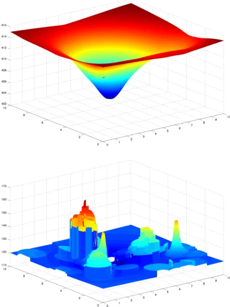
The corresponding continuous competitive facility location and design problem is the same as (1), except that M_P(x, α) is replaced by M_{P P}(x, α) as given by (2). Accordingly, its objective function will be denoted by ΠP P. It is known that (1) is a hard-to-solve global optimization problem, with many local maximum points which are not global optimal points (Fern´andez et al. 2007). The corresponding problem with the modified choice rule is even harder, as in addition to this, it also has many discontinuities. As an example, consider Figure 1, which gives the graphs of the objective function on the

Figure 1: Objective function of an instance with setting (i_max = 71, j_max = 5, k = 2) when α= 1.545898: in the top figure, using the probabilistic rule, in the bottom figure with the partially probabilistic choice rule withu= 2.

location domain for a problem with setting (i_max = 71, j_max = 5, k= 2) when the variable α is fixed to its optimal value for the partially probabilistic problem: in the top figure, using the probabilistic choice rule, and in the

0.5 1 1.5 2 2.5 3 3.5 4 4.5 5 5.5 370

375 380 385 390 395 400 405 410 415 420

0.5 1 1.5 2 2.5 3 3.5 4 4.5 5 5.5

125 130 135 140 145 150 155 160 165

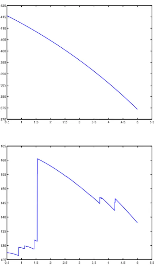
Figure 2: Objective function of an instance with setting (imax = 71, jmax = 5, k = 2) when (x1= 3.989257, x2= 7.065429): in the top figure, using the probabilistic rule, in the bottom figure with the partially probabilistic choice rule with u= 2.

bottom figure, with the partially probabilistic rule when u = 2. The white holes in the graphs correspond to the forbidden regions around the demand points. As can be seen, both problems are highly nonlinear and require global optimization techniques to be solved, although the discontinuities of the problem with the partially probabilistic choice rule, due to the capture or loss of new customers, make it much more challenging. Something similar can be seen in Figure 2, where the graphs of the objective functions are shown when the location of the new facility is fixed at the optimal location of the partially probabilistic problem. As it can be seen, whereas for the probabilistic choice rule the function is differentiable and concave with regard to α (top picture), this is no longer true for the problem with the partially probabilistic choice rule (bottom picture).

4. Solving the partially probabilistic location model

Both rigorous (Fern´andez et al. 2007) and heuristic (or incomplete) meth- ods (Redondo et al. 2009a, 2008) have been proposed to cope with the proba- bilistic model. By a rigorous method we mean a deterministic method which can obtain with certainty the global optimal solution of the problem within prescribed tolerances, even with approximate computations (see Neumaier (2004) for a taxonomy of global optimization strategies). Hence, in this sec- tion we only concentrate on the partially probabilistic model. Next, both rigorous and heuristic methods are suggested to cope with it.

4.1. A rigorous interval branch-and-bound method, iB&B

Among the rigorous methods to cope with global optimization problems, branch-and-bound (B&B) algorithms are among the most used. Their suc- cess relies on the goodness of the bounds they employ, although obtaining those bounds is sometimes a difficult task too. Interval analysis tools can be used both to compute bounds automatically (thanks to the use of in- clusion functions, see the definition below) and to speed up the process by discarding suboptimal regions (using the so-called discarding tests). The in- terested reader will find the books by Hansen and Walster (2004) and T´oth and Fern´andez (2010) very helpful. Here we just introduce some notation and a few basic concepts used later on.

The set of compact intervals will be denoted byIR, intervals in boldface letters, and lower and upper bounds of intervals by ‘underlines’ and ‘over- lines’, respectively. The width of an interval y= [y, y]∈IR will be denoted byw(y) =y−y and its relative width bywrelat(y) = w(y)/max{1,min{|y|: y ∈ y}}. The width of an interval vector y = (y₁, . . . ,y_n)^T ∈ IRⁿ (also called a ‘box’) is to be understood as w(y) = max{w(y_i) :i= 1, . . . , n}.

Definition 1. A function f : IRⁿ →IR is said to be an inclusion function for f :Rⁿ→R provided

{f(y) :y∈y} ⊆f(y) for all boxes y⊂IRⁿ within the domain of f.

Observe that iff is an inclusion function forfthen we can directly obtain lower and upper bounds of f over any box y within the domain of f, hence its usefulness in B&B methods. There exist programming languages and

libraries which have the interval arithmetic implemented (see URL (2017)), and they provide inclusion functions for predeclared functions (sin, exp,. . . ).

By using them, the natural interval extension or other techniques can be used to compute an inclusion function for other general functions (Hansen and Walster 2004, T´oth et al. 2007).

Interval B&B methods (iB&B in what follows) have been successfully applied to solve location problems (see for instance Fern´andez and Pelegr´ın (2001), T´oth and Fern´andez (2010) and the references therein). In particular, in Fern´andez et al. (2007) such an iB&B method was applied to solve the corresponding probabilistic problem described in Section 2. A similar method can handle the partially probabilistic model, thanks to the use of the interval tools employed to compute the bounds.

A point that deserves to be clarified here is how to compute an inclusion function ˜u_i0(x,α) for ˜u_i0(x, α), as this function is given by an ‘if’ condition.

This can be achieved by defining

˜

u_i0(x,α) =







0 if u_i0(x,α)< u u_i0(x,α) if u_i0(x,α)≥u h

0,u_i0(x,α)i

otherwise

where ui0(x,α) is an inclusion function for ui0(x, α). One can see that this is the cause of the discontinuity of the objective function, and it makes im- possible to use any advanced tools that use differentiability or even continu- ity inside an iB&B. Therefore, only the basic discarding tests described in Fern´andez et al. (2007) can be used for the new problem, namely, the cut- off and the feasibility tests. It is still a valuable result that a discontinuous function can be optimized by a reliable method.

The output of the method is a list of 3-dimensional boxes,L={y₁, . . . ,y_r}, which contain any global optimal solution. The best point found by the algo- rithm during its execution,y^best= (x^best₁ , x^best₂ , α^best), is also offered as output.

Let us denote by Π either Π_P or Π_{P P} depending on the problem to be solved.

Notice that any point inSr

l=1y_l will have its objective function value within the interval

[min{Π(y_l) :l = 1, . . . , r},max{Π(y_l) :l= 1, . . . , r}]

although the optimal objective function value Π^∗ of our problem is within the narrower interval

[Π(y^best),max{Π(y_l) :l = 1, . . . , r}].

The stopping rule sends a boxy to the solution listL provided that w(y)< orw_relat(Π(y))< .

In the computational studies carried out in this paper we have established that = 0.0001.

4.2. An evolutionary algorithm

In Redondo et al. (2009a), the algorithm called UEGO was proposed for solving the corresponding model with the probabilistic choice rule. In fact, it has also been applied to other competitive location problems as well (see for instance Redondo et al. (2012)). UEGO can be classified as a global evolutionary optimization method. It applies procedures based on nature on a pool of M independent candidate solutions (individuals), which form a population. In other words, it applies methods, as reproduction or selection, to address the population towards the global (or local) optima. In this sense, UEGO can also be considered as a multimodal optimization algorithm, since each candidate solution in the population is intended to occupy a local or global optimum of the fitness landscape.

Each candidate solution in UEGO represents a subspace (in fact, a hy- persphere) of the whole searching region by means of a radius. The main goal of the radius is to focus the optimization efforts on a particular sub-area.

The solution is considered to be in the center of the corresponding subspace.

During the optimization procedure, several candidate solutions with differ- ent radii can coexist simultaneously. Therefore, at the same stage of the optimization procedure, new promising regions are systematically analyzed (those with a bigger radius), while others are examined thoroughly (those with a smaller radius). The term “independent” signifies that a candidate solution has the ability of reproducing by itself, i.e. a new offspring can arise from a single individual independently of the rest of the population. It means that many peaks can be investigated in parallel and hence, the effects of the genetic drift can be prevented.

The radius associated to a candidate solution depends on the instant where it was created. Solutions created at the beginning of the search will examine big regions, while solutions created during the latest cycles will focus on smaller promising areas. More precisely, the radius of a candidate solution created at iteration i, is given by a decreasing exponential function that depends on the initial domain landscape, R₁, and an input parameter,

R_L, which represents the smallest radius. This mechanism has been designed to balance exploration and exploitation.

UEGO works as follows. Initially, a population of candidate solutions is created. The fitness is used to determine the relative merit of each individ- ual. Once the initial population is obtained, an iterative process is carried out. At each cycle, UEGO mimics natural evolution on the population by applying procedures for the reproduction of individuals, the improvement of their offspring by means of a local optimizer, and the promotion of the best candidate solutions to the next generation. As UEGO applies a local search algorithm to each individual of the population, it can be also classified as a memetic algorithm(Moscato (1989)). In fact, only the local search procedure used within UEGO needs to be adapted for each particular problem.

UEGO has four user input parameters: (i) a maximum number of func- tion evaluations for the whole optimization procedure, N; (ii) a maximum number of individuals in the population, M; (iii) a maximum number of cy- cles or iterations, L; and (iv) the radius of the smallest candidate solution R_L. The function evaluations, N, are distributed among the individuals in the population at each iteration, in such a way each one has a budget to generate new candidate solutions and to improve them. These budgets are mathematically computed by means of equations that depends on the pre- viously mentioned input parameters. See Redondo et al. (2009a) for a more detailed description of the algorithm and its parameters.

In view of its success at solving different competitive location problems, UEGO has also been adapted to the problem with the partially probabilistic choice rule. The most important adjustment consisted of selecting an appro- priate local optimizer. Initially, a Weiszfeld-like algorithm was considered as a local optimizer, following the lines in Redondo et al. (2009a). However, the obtained results were not as good as expected and it was rejected. The general purpose stochastic hill climber SASS (Solis and Wets 1981) was fi- nally included in this work, but with some modifications, which are briefly described next.

Algorithm SASS is a derivative-free optimization algorithm that can be applied to maximize an arbitrary function over a bounded subset of R^N, although internally SASS assumes that the range in which each variable is allowed to vary is the interval [0,1]. Since this is not our case, when necessary we use functions to rescale (normalize) the variable values to the interval [0,1], and to invert (denormalize) this process. In SASS, the new points are generated using a Gaussian perturbation ξ ∈ R³ over the search

point (x, α) and a normalized bias term b ∈ R³ to direct the search. The standard deviationσ specifies the size of the sphere that most likely contains the perturbation vector. In this work, its upper bound σub should have the same value than the normalized radius of the caller solution. Then, the parameterσ_ubis also considered an argument of SASS. Hence, any single step taken by the optimizer is no longer than the radius of the calling candidate solution. Finally, the stopping rules are determined by a maximum number of iterations (ic_max) and by the maximum number of consecutive failures (M axf cnt). The use of SASS as the local optimizer within UEGO has also worked fine for other location problems with discontinuities (see for instance Redondo et al. (2013)).

The parameters that control UEGO have been tuned to this new problem by trying several combinations of parameter values on a reduced set of ran- dom problems. Finally, they have been set to L = 15, R_L = 0.5, M = 100 and N = 3·10⁶.

5. On the estimation of the parameters of the model

In order to apply the location model to a particular real problem, the parameters of the model have to be estimated. Next we discuss how that estimation can be carried out.

The distances d_ij between demand points and existing facilities can be obtained directly using road maps or the shortest distance capabilities of Geographic Information Systems (GIS) or Geographic Positioning Systems (GPS). Then, with those data, a distance predicting function (DPF) can be tailored to the geographical region under consideration (Brimberg and Love 1995, Fern´andez et al. 2002), which provides an estimation of the travel distance between two points, given their geographical coordinates. That DPF can be used as d_i(x).

On the other hand, the functiongi(d) modulating the distance is usually of the form g_i(d) =d^λ org_i(d) = exp(−λd). For the simultaneous estimation of the parameter λ defining g_i(d) and the qualities of the existing facilities, ordinary least squares could be used as proposed in Nakanishi and Cooper (1974, 1982). However, the strategies proposed in Drezner (2006) or Drezner and Drezner (2002) provide similar results and are easier to implement.

The functional forms ofF and Gshould also be ascertained so that they reflect the reality as close as possible. Whereas for the income functionF this seems to be an easy task (considering the experience of the managers of the

locating chain), the functional form ofGcould be more tricky. The difficulty of the determination of those functions will depend on the particular type of facility to be installed, and on the ability and knowledge of the managers.

The estimation of the threshold values is also a critical issue, as we will see in Section 6. Using the probabilistic choice rule, the proportion of the demand concentrated at pi captured by facilityj is given by

p_ij = u_ij Pjmax

k=1 u_ik.

If we assume that whenp_ij is less than a predefined small value ˜p(for instance, let say ˜p= 0.05), then it is not ‘normal’ for a customer atp_i to go tof_j, then we can consider that the threshold for demand point p_i, denoted by u_i (the minimum level of attraction that a facility must have for the customers atp_i to spend some of his/her buying power there), lies in the interval, [u^lb_i , u^ub_i ], where

u^lb_i = max

j {u_ij :p_ij <p},˜ and u^ub_i = min

j {u_ij :p_ij ≥p}.˜

That interval can be computed easily using the available data and param- eters. However, in order to choose the value u_i ∈ [u^lb_i , u^ub_i ] that better fits the tastes of the customers at pi more information is needed. Let us denote by f_lbi the facility where u^lb_i is attained, and by f_ubi the one for which u^ub_i is attained. A survey could be carried out among the customers at demand point i asking: (i) how much closer should the facility flbi be so you would go there to buy goods or use its services?, and (ii) how much further should the facility f_ubi be so you would not go there? The average distance of the answers of each of those questions is then computed, and from those two distances, two attraction thresholds forp_i can be computed. The mean value of those thresholds could be set as u_i.

If a unique threshold valueu is required for all the demand points, then the minimum of the u_i values, or its mean, or its weighted mean could be used.

6. Probabilistic choice rule versus partially probabilistic choice rule To what extent is the difference between the probabilistic and the partially probabilistic choice rules important when deciding the location of the new facility? How much does it affect the optimal profit? We study these and

other issues first using a quasi-real example of the location of a hypermarket, and then analyzing some random problems. In both studies we will solve the same location problems using both rules, and using the exact interval branch-and-bound method mentioned in Subsection 4.1, so as to have the optimal solutions and carry out a fair comparison.

6.1. A case study

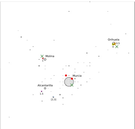
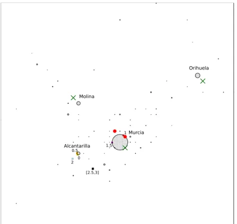
In this subsection, we investigate a quasi-real example dealing with the location of a hypermarket in an area around the city of Murcia, in south- eastern Spain. In the study, we have considered a working radius of 25 km around Murcia. 632558 inhabitants live within the circle, distributed over imax = 71 population centers. Their population varies between 1138 and 178013 inhabitants. Each population center has been considered a demand point, with buying power proportional to its total population (one unit of buying power per 17800 inhabitants), resulting the demand’s spectrum in [0.064,10]. Their location and population can be seen in Figure 3: each demand point is shown as a gray circle (or a black dot) with a radius pro- portional to its buying power. The surrounding gray circles also show the forbidden regions around the cities. Five hypermarkets are present in the area: two from a first chain A (marked with a red•), and three from another chain B (marked with a green×). Figure 3 shows the location of each hyper- market. The feasible set S was considered the smallest rectangle containing all demand points (approximately a square centered at Murcia whose sides have a length close to 45 Km).

The coordinates of the population centers and the hypermarkets were re-scaled to an approximate square ([0,10],[0,10]), in which the units corre- spond approximately to 4.5 Km. The radius of the forbidden circular area surrounding demand point p_i was set tow_i/30.

Approximate values for the quality parameters α_j for the five existing hypermarkets were obtained through a small survey among people who had visited all five hypermarkets. Each respondent was asked to rank the hy- permarkets in increasing order of their perceived quality and to indicate the difference in quality between any two consecutive hypermarkets in their ranking by a score between 1 (small) and 4 (big). That information yielded individual marks for all hypermarkets, by starting from a lowest mark of 1 and adding each difference score to obtain the mark of the next hypermar- ket in their ranking. Finally, these marks were rescaled to the interval [3,4], because, according to all the respondents, in a proposed scale from 0.5 to 5,

all considered hypermarkets have a quality above the mean (2.75). But they all still have a large margin for improvement. The qualities α_j considered are the average rescaled marks over the respondents. But see Section 5 for a better way to estimate the qualities of existing facilities in real problems.

The quality of the new facility lies in the interval [0.5,5].

For the rest of the parameters, we used the following initial settings: the income per unit of good sold c = 12, in the location cost function G₁ we chose the parameter ϕ_i0 = 2 for all i, while the value of ϕ_i1 decreases as the population increases. Finally, the parameters of the quality cost functionG2

were initially set to β₀ = 7 and β₁ = 3.75. The interested reader is referred to T´oth et al. (2009) for more details about this example.

Three different scenarios have been considered:

1. Scenario ‘small chain A’: The locating chain is the small one, chain A, which owns k = 2 of thejmax = 5 existing facilities.

2. Scenario ‘large chain B’: The locating chain is the greatest one, chain B, which owns k = 3 of the 5 existing facilities.

3. Scenario ‘newcomer’: The locating chain is new in the market (k = 0), and the new facility will have to compete with the 5 existing facilities.

The following notation will be used when analyzing the results: Π_P(·) is the objective function of location problem (1) when the probabilistic choice rule is employed, LP gives the output list of 3-dimensional boxes which con- tain any optimal solution, and (x^∗_P, α_P^∗) represents the best point found by the algorithm during the execution. The corresponding items for the problem with the partially probabilistic choice rule will be denoted by Π_{P P}(·), LPP

and (x^∗_{P P}, α^∗_{P P}).

We will compute the Euclidean distance between the locations x^∗_P and x^∗_{P P}, which is denoted as dist_loc, as well as the absolute difference between the qualities α^∗_P and α^∗_{P P}, denoted as dist_qual, to measure the difference between the optimal solutions.

The objective function value of the partially probabilistic model before (Π_{P P}(before)) and after (Π_{P P}(x^∗_{P P}, α^∗_{P P})) the location of the new facility will be shown, as well as the cost due to the new facility, G(x^∗_{P P}, α^∗_{P P}). We will compute the relative profit loss incurred when the probabilistic choice rule is assumed in a problem where the partially probabilistic rule should have been chosen,

lost(P|P P) = 100·(Π_{P P}(x^∗_{P P}, α^∗_{P P})−Π_{P P}(x^∗_P, α^∗_P))/Π_{P P}(x^∗_{P P}, α^∗_{P P}),

and the relative profit loss incurred when the partially probabilistic choice rule is assumed in a problem where the probabilistic rule should have been chosen,

lost(P P|P) = 100·(Π_P(x^∗_P, α^∗_P)−Π_P(x^∗_{P P}, α^∗_{P P}))/Π_P(x^∗_P, α^∗_P), to measure the cost of choosing the inadequate model for the chain as a whole.

Similarly, to measure the cost of choosing the inadequate model in the profit increment due to the new facility, the relative profit lost due to the new facility only when the probabilistic choice rule is assumed in a problem where the partially probabilistic rule should have been chosen,

lost(P|P P)₀ = 100· IncrΠ_{P P}(x^∗_{P P}, α^∗_{P P})−IncrΠ_{P P}(x^∗_P, α^∗_P) IncrΠP P(x^∗_{P P}, α^∗_{P P}) ,

will be computed, whereIncrΠ_{P P}(x^∗_{P P}, α^∗_{P P}) = Π_{P P}(x^∗_{P P}, α_{P P}^∗ )−Π_{P P}(before) andIncrΠ_{P P}(x^∗_P, α^∗_P) = Π_{P P}(x^∗_P, α^∗_P)−Π_{P P}(before).Analogously,lost(P P|P)₀ will be computed too. For the newcomer case these two values are not com- puted, as they coincide with lost(P|P P) and lost(P P|P), respectively.

As the demand actually served by the facilities may vary depending on the threshold value u employed (remember that we may have unmet demand), we will also compute the percentage of the total demand really served before (%W_{T B}) and after (%W_{T A}) the location of the new facility, the percentage of the total demand captured by the locating chain before (%WCB) and after (%W_CA) the new facility is located, and the percentage of the total demand captured by the new facility (%W_new). Notice that %W_CB+ %W_new may be different from %WCA, since the new facility may steal part of the demand to the existing chain-owned facilities (an effect known as cannibalization). The total demand in the region in all the cases isW =Pimax

i=1 w_i = 35.53. For the newcomer case, %WCB and %WCA are omitted, as the locating chain has no existing facilities. For the sake of completeness, we also show the quality of the new facility for each value of u.

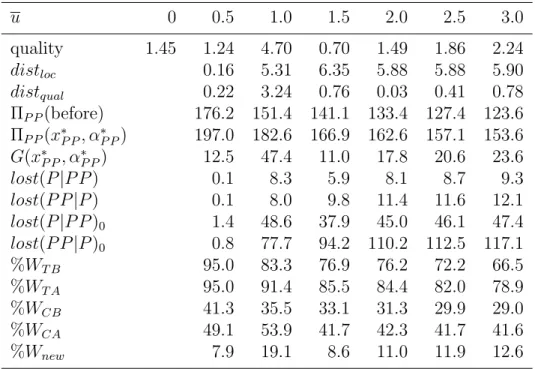
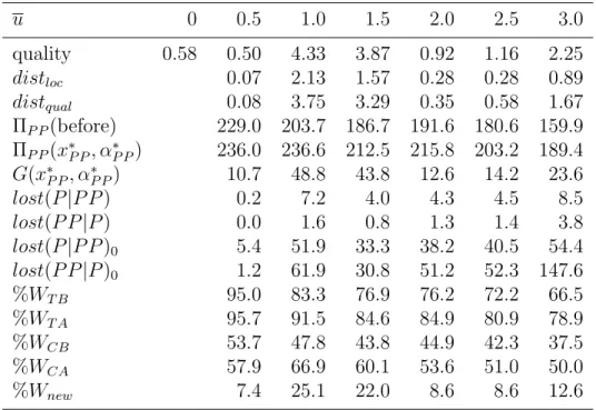
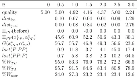
The results obtained for each of the three scenarios are shown in tables 1, 2 and 3, respectively.

As we can see, in the scenario ‘small chain A’ (see Table 1), even for the threshold u = 0.5 (a small value with which 95% of the total demand is still served) we can observe that both the location and the quality of the new facility to be located are different from those of the probabilistic choice

[2,3]

0 0.5

1

1.5

Murcia Alcantarilla

Molina

Orihuela

Figure 3: Case study: scenario small chain A.

rule (see Figure 3, where the optimal locations for the different values of u are drawn as small squares in different colors). However, the differences are not too important, as the optimal solution is still to locate the new facility close to Orihuela, the second most populated city, in the North-East of the map, where one of the facilities of the competing chain is set up (the chain already has two facilities in the surroundings of the most populated city, Murcia, so this is not the optimal place to expand the chain, due to the cannibalization). In fact, the differences in objective function value are almost negligible. It is for u= 1 where we can observe a big change, both in location and quality. In this case, the optimal location changes to the third most populated city, Molina (in the North-West of the map, where another facility of the competing chain operates). The reason is that Molina is closer to Murcia, and the new facility not only competes against the competitor’s

Table 1: Case study: differences in the solutions obtained by the probabilistic and the partially probabilistic choice rules for the scenario ‘small chain A’.

u 0 0.5 1.0 1.5 2.0 2.5 3.0

quality 1.45 1.24 4.70 0.70 1.49 1.86 2.24

dist_loc 0.16 5.31 6.35 5.88 5.88 5.90

dist_qual 0.22 3.24 0.76 0.03 0.41 0.78

Π_{P P}(before) 176.2 151.4 141.1 133.4 127.4 123.6 Π_{P P}(x^∗_{P P}, α^∗_{P P}) 197.0 182.6 166.9 162.6 157.1 153.6 G(x^∗_{P P}, α^∗_{P P}) 12.5 47.4 11.0 17.8 20.6 23.6

lost(P|P P) 0.1 8.3 5.9 8.1 8.7 9.3

lost(P P|P) 0.1 8.0 9.8 11.4 11.6 12.1

lost(P|P P)₀ 1.4 48.6 37.9 45.0 46.1 47.4 lost(P P|P)₀ 0.8 77.7 94.2 110.2 112.5 117.1

%WT B 95.0 83.3 76.9 76.2 72.2 66.5

%W_{T A} 95.0 91.4 85.5 84.4 82.0 78.9

%W_CB 41.3 35.5 33.1 31.3 29.9 29.0

%WCA 49.1 53.9 41.7 42.3 41.7 41.6

%W_new 7.9 19.1 8.6 11.0 11.9 12.6

facility in Molina, but also attracts part of the demand from Murcia and Alcantarilla (the fourth most populated city), thanks to its high quality.

Notice that when the facility is located in Orihuela, if u = 1, even a high quality is not enough to attract demand from Murcia. As can be seen in Table 1, when u = 1 an inadequate choice in the patronizing behavior of customers may lead to a considerable relative profit lost of around 8%. In fact, in this case the new facility captures 19.1% of the total demand, more than 1/3 of the demand captured by the chain. When u = 1.5 we can observe another change in the location, which moves to the South-West, close to Alcantarilla and closer to Murcia; now the quality of the new facility is small, which reduces the costs, but still allows to capture most of the demand from Alcantarilla and its surroundings. Finally, foru= 2, 2.5 and 3 a final change can be observed, where the location is the same for all those values, and only the quality changes. Now, although the new facility is at a similar distance from the most populated city, it is set up in a cheaper

place and it is closer to the competitor’s facility in Murcia, which allows to compete against it and to capture part of the demand from the South-West area (although at the cost of a higher quality.

Note that an increase in the market share captured does not necessarily means an increase in the profit, since the increment in the market share captured can be due to a higher quality or a better and more expensive location, and in both cases this implies a higher cost, and maybe the cost exceeds the income obtained from the market share captured. For instance, from u =0.5 to 1.0 the chain capture more market share (from 49.1% to 53.9%, which is an increase of 9.77%), but the profit decreases (from 197.0 to 182.6, a 7.30%) since the cost due to the new facility increases from 12.5 to 47.4, mainly due to the increment in the quality (from 0.22 to 3.24).

[2.5,3]

2

1.5 1

0.5 0

Orihuela

Molina

Murcia Alcantarilla

Figure 4: Case study: scenario large chain B.

In the scenario ‘large chain B’, for both the probabilistic choice rule (u=

Table 2: Case study: differences in the solutions obtained by the probabilistic and the partially probabilistic choice rules for the scenario ‘large chain B’.

u 0 0.5 1.0 1.5 2.0 2.5 3.0

quality 0.58 0.50 4.33 3.87 0.92 1.16 2.25

dist_loc 0.07 2.13 1.57 0.28 0.28 0.89

dist_qual 0.08 3.75 3.29 0.35 0.58 1.67

Π_{P P}(before) 229.0 203.7 186.7 191.6 180.6 159.9 Π_{P P}(x^∗_{P P}, α^∗_{P P}) 236.0 236.6 212.5 215.8 203.2 189.4 G(x^∗_{P P}, α^∗_{P P}) 10.7 48.8 43.8 12.6 14.2 23.6

lost(P|P P) 0.2 7.2 4.0 4.3 4.5 8.5

lost(P P|P) 0.0 1.6 0.8 1.3 1.4 3.8

lost(P|P P)₀ 5.4 51.9 33.3 38.2 40.5 54.4 lost(P P|P)₀ 1.2 61.9 30.8 51.2 52.3 147.6

%WT B 95.0 83.3 76.9 76.2 72.2 66.5

%W_{T A} 95.7 91.5 84.6 84.9 80.9 78.9

%W_CB 53.7 47.8 43.8 44.9 42.3 37.5

%WCA 57.9 66.9 60.1 53.6 51.0 50.0

%W_new 7.4 25.1 22.0 8.6 8.6 12.6

0) and the partially probabilistic choice rule with threshold value u = 0.5, the optimal solution is to locate the facility close to Alcantarilla, the fourth most populated city, with a very small quality: since there exist no other facilities around, the new facility captures most of its demand (see Figure 4) with a low cost.

However, when u = 1 the optimal location moves to the surroundings of Murcia, the most populated city, between the two existing facilities of the competing chain, and this, despite the fact that the chain already owns a facility in the South-East of that city; to compete against them, a high quality is required. Notice that withu=0.5, the total market share served before the location of the new facility was 95.0%; whereas with u=1.0 it is only 83.3%.

This means that part of the demand at Murcia (and other cities around) is not served by the existing facilities, and so, there is an opportunity for the new facility to capture that unserved demand. In fact, after the location of the new facility, the total demand served increases to 91.5%. As we can see,

in this case, lost(P|P P) = 7.2%, a very high value taking into account that the locating chain is dominant in the market and that 91.5% of the total demand is served after the location of the new facility. In this case, the new facility captures 25.1% of the total demand, whereas the chain, considering all the facilities, gets 66.9% of the total demand, i.e., the new facility captures 37.5% of the demand of the chain. This is, however, at the expense of suffering some cannibalization: notice that %W_CB + %W_new = 72.9%, more than %W_CA = 66.9%. When u= 1.5 the optimal location moves to another part of the city of Murcia, far from the existing competing facilities, which allows the reduce the quality, and hence, the costs, but still capturing a good part of the demand at Murcia, even though suffering some cannibalization.

When u=2.0 the location changes again, close to Alcantarilla, again with a low quality. Since the costs are again much smaller, the profit increases, and this despite capturing a smaller percentage of the market. And finally, for u= 2.5 and 3, a new location is obtained, similar to that of the small chain scenario, not too close to Murcia nor to Alcanrilla to reduce the location costs (see Figure 4), and with a medium quality. Notice that, as expected, the cannibalization decreases as u increases.

Table 3: Case study: differences in the solutions obtained by the probabilistic and the partially probabilistic choice rules for the scenario ‘newcomer’.

u 0 0.5 1.0 1.5 2.0 2.5 3.0

quality 5.00 5.00 4.92 4.16 4.37 5.00 2.24

dist_loc 0.10 0.67 0.04 0.01 0.09 1.29

dist_qual 0.00 0.08 0.84 0.62 0.00 2.76 ΠP P(before) 0.0 0.0 -0.0 0.0 0.0 0.0 Π_{P P}(x^∗_{P P}, α^∗_{P P}) 45.6 60.9 52.2 50.6 43.3 30.1 G(x^∗_{P P}, α^∗_{P P}) 56.7 55.7 46.8 49.3 56.6 23.6 lost(P|P P) 0.9 11.8 3.7 4.1 45.0 17.4 lost(P P|P) 0.7 5.8 3.8 2.3 10.2 64.5

%W_{T B} 95.0 83.3 76.9 76.2 72.2 66.5

%WT A 95.7 91.5 84.6 83.4 80.8 78.9

%W_new 24.0 27.3 23.2 23.4 23.4 12.6

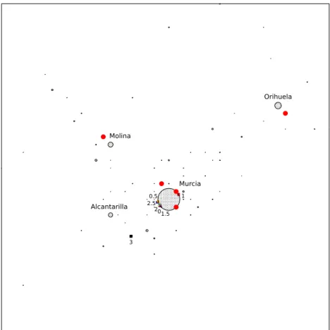
Concerning the ‘newcomer’ case, for u= 0 to 2.5, the optimal solution is

1

3

201.5 2.5

0.5

Orihuela

Molina

Murcia Alcantarilla

Figure 5: Case study: newcomer.

to locate the new facility in the surroundings of Murcia, the most populated city (see Figure 5). Even though there already exist three facilities around Murcia and there will be fierce competition, for the newcomer it is still the best option, as most of the demand is concentrated there. A high quality is required, though. It is important to highlight, however, that even with very small differences in location and quality, the relative profit loss incurred when an inadequate patronizing behavior of customers is assumed may be very high. See for instance the caseu= 2.5. In this case, the difference in location is very small (dist_loc = 0.09) and the difference in quality with regard to the probabilistic case is almost negligible. Nevertheless, lost(P P|P) = 10.2%

and lost(P|P P) = 45.0%. This clearly shows the big difference between the probabilistic and the partially probabilistic choice rule. For u = 3 the

relative profit lost is even higher, although in this case the location moves to a different place, the same as that of the small and large chain scenarios whenuis 2.5 or more (not too close to Murcia nor to Alcanrilla to reduce the location costs), and the quality is also different from that of the probabilistic case. In this case, since u is very high, none of existing facilities can capture the demand from Alcantarilla and the cities around, and the new facility can capture it, and with a low quality and in a cheap location.

Summarizing, we can see that both the location and/or the quality of the facility to be located may change drastically as the threshold value varies, and even when those changes are very small, the relative profit loss incurred for the chain when an inadequate choice rule is employed may be very high.

This is due to discontinuities of the objective function, see figures 1 and 2:

every time a new demand point is captured or lost (and this may happen with a small change in the location and/or the quality), a jump in the objective function happens. This clearly shows that the selection of the choice rule in competitive location models should be made with care, and the assumption of the probabilistic choice rule commonly done in literature should only be considered when it is really the case.

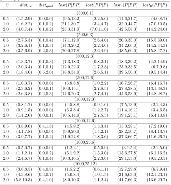
6.2. Random problems

We have done a similar study on a set of 40 random problems, half of them withn= 500 demand points and the rest with 1000 demand points, although in this case, for the sake of brevity, only the differences in the location, quality and objective value have been analyzed. Several settings (i_max, j_max, k) have been considered (see Table 4), and for each of them, five problems were generated by randomly choosing the parameters of the problems uniformly within the following intervals:

• p_i, f_j ∈S,

• ω_i ∈[0,100/√ n],

• αj ∈[0.4,6],

• G(x, α) =Pimax

i=1 Φ_i(d_i(x)) +G₂(α) where

• Φ_i(d_i(x)) = w_i(d ¹

i(x))^ϕi0+ϕi1 with ϕ_i0 =ϕ₀ = 2, ϕ_i1 ∈[0.5,1.5],

• G₂(α) =e^βα0+β1−e^β1 with β₀ ∈[7,9], β₁ ∈[6,6.5],

Table 4: Random problems: differences in the solutions obtained by the probabilistic and partially probabilistic choice rules.

u distloc distqual lost(P|P P) lost(P P|P) lost0(P|P P) lost0(P P|P) (500,6,1)

0.5 (1.5,2.9) (0.0,0.0) (9.5,13.2) (2.2,5.6) (14.6,21.7) (4.0,8.7) 1.0 (1.6,2.2) (0.1,0.2) (21.1,30.7) (3.4,4.7) (32.0,44.7) (7.0,10.5) 2.0 (4.0,7.4) (0.1,0.2) (25.3,31.0) (7.0,11.6) (42.5,58.3) (14.2,24.0)

(500,6,3)

0.5 (2.7,5.3) (0.1,0.4) (7.1,12.0) (2.6,4.0) (20.3,35.0) (15.5,39.0) 1.0 (3.2,6.1) (0.1,0.3) (14.3,20.2) (2.2,4.6) (34.2,66.0) (14.2,44.3) 2.0 (3.5,6.9) (0.2,0.3) (20.0,27.8) (2.6,4.9) (48.5,60.0) (15.8,47.2)

(500,12,3)

0.5 (1.3,3.7) (0.1,0.3) (7.3,18.3) (0.8,2.1) (18.3,39.2) (4.2,14.9) 1.0 (2.0,3.4) (0.1,0.1) (12.0,22.3) (1.7,2.3) (25.9,33.5) (6.7,9.8) 2.0 (1.8,4.0) (0.5,2.0) (18.8,34.0) (2.6,5.1) (39.5,50.3) (9.5,14.4)

(500,12,6)

0.5 (1.6,3.7) (0.0,0.0) (5.8,8.8) (1.0,2.2) (16.7,26.7) (6.4,16.7) 1.0 (2.3,6.2) (0.0,0.1) (10.0,15.1) (2.7,8.5) (27.8,38.5) (13.1,38.3) 2.0 (2.6,3.8) (0.2,0.3) (14.6,20.3) (2.7,4.1) (44.6,53.9) (14.8,28.2)

(1000,12,3)

0.5 (0.8,1.2) (0.0,0.0) (4.5,8.8) (0.9,1.6) (7.5,13.9) (2.2,4.3) 1.0 (0.9,1.5) (0.0,0.0) (6.3,8.4) (1.2,2.7) (11.4,16.1) (3.4,6.5) 2.0 (1.4,2.0) (0.0,0.1) (10.5,14.0) (2.7,5.3) (19.1,25.1) (6.4,10.8)

(1000,12,6)

0.5 (3.8,9.0) (0.4,1.8) (4.5,9.2) (1.3,3.4) (15.0,28.1) (7.2,19.0) 1.0 (4.1,7.8) (0.0,0.0) (9.9,20.0) (1.4,2.1) (28.2,50.7) (8.4,13.7) 2.0 (3.9,7.7) (0.1,0.2) (11.9,24.8) (1.8,3.6) (37.3,66.7) (11.6,26.2)

(1000,25,6)

0.5 (0.5,0.7) (0.0,0.0) (1.2,2.1) (0.5,0.9) (3.1,5.4) (2.2,5.0) 1.0 (1.1,2.1) (0.0,0.2) (5.1,9.2) (1.5,3.0) (13.6,27.8) (6.1,16.2) 2.0 (2.4,6.7) (0.1,0.4) (10.3,16.5) (2.2,3.6) (29.1,53.3) (9.5,20.5)

(1000,25,12)

0.5 (3.6,8.5) (0.4,0.8) (1.5,2.2) (0.6,1.1) (12.7,29.8) (6.7,9.4) 1.0 (4.3,8.6) (0.3,0.7) (5.0,8.4) (1.0,1.5) (31.6,63.0) (12.1,23.1) 2.0 (5.8,10.3) (0.4,1.0) (8.0,10.3) (1.1,2.4) (41.7,66.3) (13.6,29.7)

• c∈[10,11], the parameter for F(M(x, α)) =c·M(x, α),

The meaning of the columns in Table 4 correspond to those of tables 1, 2 and 3. For each setting and each threshold value u, the average value of the five problems, followed by the corresponding maximum, are given.

As we can see, even for u = 0.5 we have instances where the relative