Solving ordinary differential equation systems by approximation in a graphical way

(2006) pp. 57–68

http://www.ektf.hu/tanszek/matematika/ami

Solving ordinary differential equation systems by approximation in a

graphical way

Gábor Geda

, Anikó Vágner

aDepartment of Computer Science Eszterházy Károly College e-mail: gedag@aries.ektf.hu

bDepartment of Information Technology Eszterházy Károly College e-mail: vagnera@aries.ektf.hu

Submitted 11 November 2006; Accepted 18 December 2006

Abstract

Our aim was to find a graphic numeric solution method for higher-order differential equations and differential equation systems. To understand this method the basic mathematical knowledge taught in the secondary school must be enough, we have to complete it with geometric meaning of differential quotient and generalization of knowledge about two-dimensional vector space.

We considered it important to make this method easy to algorithm. Such method and its practical experience are shown in this paper.

MSC:65L05, 65L06, 53A04,97D99

1. Introduction

It is well-known how important the differential equation models are in the math- ematical description of different processes and systems.

Our aim is to find approximate methods which are based on the demonstration and there is no need for higher mathematical knowledge to understand and apply them. Moreover, it is easy to algorithmise them even in the possession of the secondary school material.

The problem concerning this topic such as mechanical oscillations can be given as an ordinary n-order differential equation:

57

y⁽ⁿ⁾(t) =g(t, y(t), y⁽¹⁾(t), y⁽²⁾(t), . . . , y⁽ⁿ⁻¹⁾(t))

This can be transformed to explicit ordinary differential equation system (ab- breviated as ODES in the followings):

˙

xi(t) =fi(t, x1(t), x2(t), . . . , xn(t)) (i= 1, . . . , n). (1.1) The solution for these equations, if it exist at all, can be given with xi(t) (i = 1, . . . , n) functions. In most cases to produce such solutions is a difficult task which needs the knowledge of serious mathematical devices.

We consider the solutionsn+ 1-dimensional space curve x(t) = (t, x1(t), x2(t), . . . , xn(t)).

So (1.1) corresponds a vector to any point in n+ 1-dimensional vector place, and the vector is parallel with the tangent line at a givenP point of the solution of ODES. The only problem is that we do not know which points should be considered belonging to the same curve among the points close to one another.

In certain cases there is no need to present all the possible solutions, that is all curves, only the x(t)curve is necessary of which a given

P0(p0;p1;p2;. . .;pn) fits, and on the coordinates of which

xi(p0) =pi (i= 1, . . . , n)

is realized. In this case we can say that we solve an initial value problem. By expressing an initial value problem we choose one of the curves which are solutions for ODES. Other times we have to be contented with the approximate solution of the problem.

In a geometrical point of view the solution for an initial value problem by approximation is giving a P0, P1, . . . , Pk point serial the elements of which fit to the chosen curve by desired accuracy. The serial of points (06i6k) determines a broken line the points of which approximate well the points of the curve.

The accuracy of the approximation is influenced by several factors. The most important ones among them are the approximate algorithm and ODES itself.

This way, when we select the successive elements of the point serial we should take the changes of the curve of the function into consideration.

2. Demonstration of an approximate method

Let (1.1),

P0(p0;p1;p2;. . .;pn)

point on coordinates of which

xi(p0) =pi (i= 1, . . . , n)

is realized and a suitable minor d distance. We would like to determine the broken line running through P0 point and approaching the

x(t) = (t, x1(t), x2(t), . . . , xn(t))

function curve meaning the solution in the surroundings ofP0given point.

Letm^pvector be parallel with tangent line to curves atP0point. The coordi- nates ofm^pare:

m^p₀= 1

m^p_i = ˙xi(p0) (i= 1, . . . , n).

Define pvector, wherepis parallel withm^p vector andkpk=d, that is p= m^p

km^pkd. (2.1)

O

Q P

C

P

1

p

1

1

q

c

c

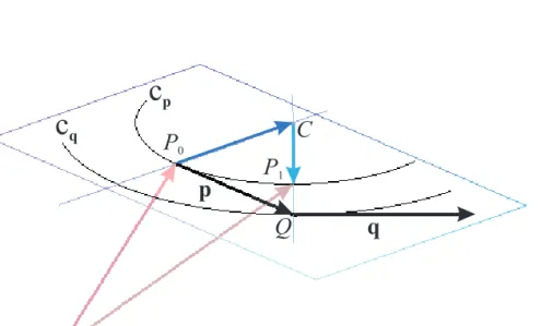
Figure 1: Thecpand thecq osculation circles in casen= 2(in 3 dimension)

DefineQpoint, where−−→

P0Q=p. Then coordinates ofQpoint can be calculated (see figure 1). Let coordinates ofQpoint beQ(q0;q1;. . .;qn).

Coordinates of m^q vector, which is parallel with tangent line to curves at Q point is:

m^q₀= 1

m^q_i = ˙xi(q0) (i= 1, . . . , n).

Ifdis minor enough, thenQis close enough to the curve which is the solution for the initial value problem. This way, m^q well approximates the steepness of the curve in one of its points near toQ.

Defineqvector, whereqis parallelm^q vector andkqk=d, in other words q= m^q

km^qkd. (2.2)

If qvector is parallel with pvector, then we acceptQ point as the next element of serial of points, and we continue the approaching from this point.

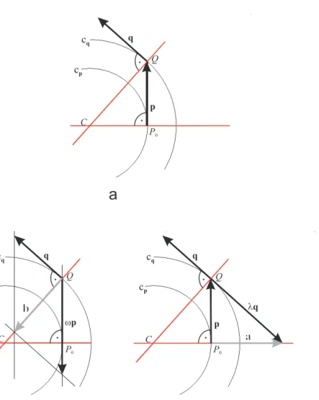
Otherwise in the narrow surroundings ofP0the curve can be well approximated in the plane, which p and q vectors define with a proper arc (cp), which is the osculating circle of the curve in P0. Similarly, we can fit an arch (cq) in (p,q) plane in the narrow surroundings ofQto the curve on whichQfits (see figure 2.a).

The lines which are perpendicular tangent lines in P0 and Q points intersect at pointC. This point can be considered to be the common central point of the two circles (cpandcq) if thedis minor enough.

Define a and bvectors for coordinates of C point: a =p+λq, and let a be perpendicular topvector, andb=q+ωpand letbbe perpendicular toqvector (see figure 2.b; 2.c).

Aspand aare perpendicular to each other, their scalar product is null, from whichλcan be calculated:

λ=− Pn

i=0p²_i Pn

i=0piqi

.

Similar way, can we get value ofω from scalar product ofqandb:

ω=− Pn

i=0q²_i Pn

i=0piqi

.

On the one hand, −−→

OC local vector can be written with −−→

OP0 local vector and a vector multiplies by a constant, on the other hand, with −−→

OQ local vector and b vector multiplied by an other constant. That is:

−−→OC=−−→

OP0+φa=−−→

OP0+φp+φλq, (2.3)

−−→OC=−−→

OQ+ψb=−−→

OQ+ψq+ψωp. (2.4)

We know, that

−−→OQ−−−→

OP0=p.

Then in the(p,q)base are the value ofφandψcan be calculated:

φ= 1

λω−1; ψ= λ

λω−1. (2.5)

C

P0

Q q

1p

a

c_p c_q

C

P₀ Q q

wp

1b

C

P0

Q q

1p

lq

1a

-b -c

c_p c_q

c_p c_q

Figure 2: Thecp andcq osculation circles in the plane ofpandq

Then coordinates of Cpoint can also be calculated in both(p,q)base andn+ 1- dimensional vector place.

Knowing coordinates ofC point we can defineP1 point, as a point of the line defined byC andQpoints and ofcp arc, namely−−→

CP1 vector is parallel with−−→

CQ vector,

−−→CP1

=

−−→CP

andP1point is on theCQhalf-line. So

−−→OP1=−−→

OP0+−−→

P0C+−−→

CP1, where−−→

OP0 and−−→

OP1 are local vectors (see figure 1).

To determine the following approximate point, the starting point will beP1 as it wasP0earlier.

The promptness of the approximation depends on the selection of the valued.

If it is too big, C will not be a good approximation of the common centre of the two osculating circles (cp andcq).

At the same time, if we find an appropriateCpoint then the distance ofCand P0approximate the radius of the circle of curvature atP1. This can be used to get a better defining of the value ofd. If we can choose the value ofdaccording to the characteristics of the curve we can approximate the function more precisely, and the algorithm will be faster.

To understand the operation of this method we only need the knowledge of graphic meaning of the differential quotient as the exact definition is not used in this case.

If we regard an ODES as a function which orders vector to the point ofn+ 1- dimensional place, where the vector is parallel with the tangent line at the point then the point serial giving the solution can be written by the use of vector op- eration based on the method mentioned above (in the followings OCM–osculating circle method) which approximates the solution of initial value problem.

To give the algorithm we need the knowledge of the equation system and vector operations (such as scalar product, vector addition).

3. Look at the problem in case n = 2

Let the next initial value problem be given

˙

x1(t) =f1(t, x1(t), x2(t)),

˙

x2(t) =fi(t, x1(t), x2(t)), P0(p0;x1(p0);x2(p0)).

The solution of initial value problem is thex(t) = (t, x1(t), x2(t))curve, which can be approximated with P0, P1, . . . , Pk serial of points. The m^p(1,x˙1(p0),x˙2(p0)) vector is parallel with tangent line of the curve atP0 point. Then coordinates ofp vector can be calculated on grounds (2.1).

If coordinates of Q point areQ(q0;q1;. . .;qn)thenm^q(1,x˙1(q0),x˙2(q0))is the vector belonging to Q. From m^q coordinates of q vector are calculatable ground of (2.2). Value ofλandω can be defined:

λ=− p²₀+p²₁+p²₂ p1q1+p1q1+p2q2

,

ω=− q₀²+q₁²+q²₂ p1q1+p1q1+p2q2

.

Ground of these considering (2.3), (2.4) and (2.5) coordinates ofCpoint can be calculatable, from which coordinates ofP1 are also calculatable grounding of−−→

CP0,

−−→CQvectors and

−−→OP1=−−→

OP0+−−→

P0C+−−→

CP1

vector.

4. Examples

To illustrate the usefulness of algorithm we show two examples. Data for the figures of the examples were provided by a program, which was made on the base of above demonstrated algorithm. The initial values and parameters can be chosen randomly, the values in the examples provide the demonstration of working of algorithm. The aim was not to show the mathematical model.

4.1. Equation of damped oscillation

Generally:

x⁽²⁾(t) + c

mx⁽¹⁾(t) +ω²x(t) = 0,

where c, m and ω are constants characteristic of the system. We get the next equation system after transforming:

˙

x1(t) =x2(t),

˙

x2(t) =−c

mx2(t)−ω²x1(t).

Choosec= 1,m= 2andω=πin the example. Then

˙

x1(t) =x2(t),

˙

x2(t) =−1

2x2(t)−π²x1(t). (4.1) Define the approximated solution of equation system where the initial conditions are

x1(0) = 0.28 x2(0) = 0.28 values by using OCM algorithm.

Compare our solution to numeric solution produced by Runge-Kutta4 method of Maple program. In both methods we have approximated the solution (h= 350).

Figure 3: Curve of meaning the solution of (4.1) equation system.

OCM RK 4 Amplitude (X )1

.t

Figure 4: Deflection-time function.

4.2. Lotka-Volterra model

Lotka-Volterra equations are suitable for modelling various occurrences, systems for examples ecological systems, chemical processes. The model can be defined with next equations:

˙

x1(t) =−ax1(t) +bx1(t)x2(t)−mx²₁(t),

˙

x2(t) =cx1(t)−dx1(t)x2(t)−lx²₂(t).

The actual entity number of predatory isX1, prey isX2. a, b, c, d, m, lare constant characteristic of the system. In our example we examine the system a = 2; b = 0.015;c= 1;d= 0.03;m= 0; l= 0.0005:

˙

x1(t) =−2x1(t) + 0.015x1(t)x2(t),

˙

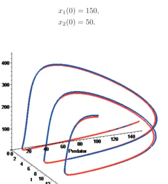
x2(t) =x1(t)−0.03x1(t)x2(t)−0.0005x²₂(t). (4.2) Initial condition is:

x1(0) = 150, x2(0) = 50.

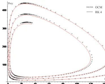
Figure 5: Curve meaning the solution of (4.2) equation system.

OCM RK 4

Predator Prey

Figure 6: Trajectory of (4.2).

OCM RK 4

Predator Prey

Figure 7: Change of entity number of predators and preys in time.

5. Conclusion

In case of various approximating method the solution can be approximated more precisely by increasing of the applied basis points. But this makes the method more difficult and needs more counting. Despite OCM, considers two basis points, the method provides comparatively great precision. It can be explained by approxi- mating the curve on short periods with arcs. The curve piece, which is between any definite two basis points, can be approximated with an arc with suitable radius, in other words, any point on the curve piece between Pi, Pi+1 points can be ap- proximated with a suitable point of arch. Giving the solution by vector equation, despite we give in n+ 1dimensional vector space, can be easy. As we reduce the solution to a 2-dimensional case, we can avoid the solution of equation system, which has more equation than two.

References

[1] Geda, G.,Solving initial value problem by different numerical methods: Practical investigation,Annales Mathematicae et Informaticae(2005).

[2] Geda, G., Solving Initial Value Problem by Approximation in Different Graphic Ways,5^thIntrnational Conference of PhD Students, Miskolc(2005).

[3] Arató, M.A Famous Nonlinear Stocshastic Equation (Lotka-Volterra Model with Diffusion),Mathematical and Computer Modelling, (2003).

[4] Geda, G.Investigation of Stability of Nonlinear Differential Equations with Stochas- tic Methods,XXVI. Seminar on Stability Problems for Stochastic Models, (2005).

[5] Stoyan, G., Tako, G.,Numerikus módszerek,ELTE-TypoTEX, Budapest, (1993).

[6] Hatvani, L., Pintér, L., Differenciálegyenletes modellek a középiskolában, POLYGON, Szeged, (1997).

[7] Rontó, M., Raisz, Péterné., Differenciálegyenletek műszakiaknak, Miskolci Egyetemi Kiadó, Miskolc, (2004).

[8] Szőkefalvi-Nagy Gy., Gehér L., Nagy P., Differenciálgeometria, Műszaki Könyvkiadó, Budapest,, (1979).

[9] Geda, G., Kezdetiérték-probléma közelítő megoldásának egy geometriai szemlél- tetése,Tavaszi Szél, Debrecen, (2005).

[10] Pólya, Gy., Matematikai módszerek a természettudományban, Gondolat, Bu- dapest, (1984).

Gábor Geda

Department of Computer Science Eszterházy Károly College Leányka str. 6.

H-3300 Eger, Hungary Anikó Vágner

Department of Information Technology Eszterházy Károly College

Leányka str. 6.

H-3300 Eger, Hungary