32(2005) pp. 203–210.
Solving initial value problem by different numerical methods: Practical investigation
Gábor Geda
Department of Computer Science, Eszterházy Károly College e-mail: gedag@aries.ektf.hu
Abstract
Our aim was to study what kind of bases can be provided to understand the basic terms of differential equation through teaching mathematical mate- rial in secondary school and to what extent this basis has to be expanded so that we can help the demonstration of differential equation. So if we give up the usual expansion of mathematical device we have to find another method which is easy to algorithmise and lies on approach. Such method and its practical experience are shown in this paper.
AMS Classification Number: 65L05, 65L06, 53A04, 97D99
1. Introduction
It is well-known how important the differential equation models are in the mathematical description of different processes and systems. Our aim is to find approximate methods which are based on the approach and there is no need for higher mathematical knowledge to understand and apply them. Moreover, they are easy to algorithmise even in the possession of the secondary school material.
The problems, concerning this topic can be given as an explicit first-order ordinary differential equation (abbreviated as ODE in the followings).
y0=f(x, y(x)) (1.1)
The solutions for these equations (if they exist at all) are y(x) functions. In most cases to give such a function is a difficult task which needs the knowledge of serious mathematical devices. Starting from the side of approach we can say that by giving (1.1) we give the slope of those tangents which can be drawn to all points of the curves of the functions providing the solution. So (1.1) correspond a given steepness to points of the place, the value of the steepness of tangent taken
203
Other times we have to be contented with the approximate solution of the problem. In a geometrical point of view the solution for an initial value problem by approximation is giving a P0, P1,. . . , Pn point serial the elements of which fit to the chosen curve by desired accuracy. The serial of vectors−−→
PiPi+1 (05i < n) determines a broken line the points of which approximate well the points of the curve. The accuracy of the approximation is influenced by several factors. The most important ones among them are the approximate algorithm and ODE itself.
This way, when we select the successive elements of the point serial we should take the changes of the curve of the function into consideration.
2. Demonstration of an approximating method
Let ODE (1.1), P0(x0,y0) be given and minor d distance. We would like to determine the broken line running through a given point and giving the function curve in the surroundings of a given point.
m0=f(x0, y0)is the steepness of a tangent belonging to point P0. Let~abe a vector parallel with line ofm0 steepness and k~ak=d. Define point Q(x,y) where
−−→P0Q=~a(see Figure 1). Steepness (m) belonging to Q can also be calculated.
Ifd is minor enough, then Q is close enough to the curve which is the solution for the initial value problem. This way,m well approximates the steepness of the curve in one of its points near to Q.
Let~b be a vector parallel with the tangents the steepness of which is m and k~bk=d, and in addition, we must chose the direction of~bin a way, that the angle of~aand~bmust be equal with the angle of lines withm0 andm steepness.
In the narrow surroundings of P0the curve of the function can be well approx- imated with a proper arc (c2) which is the circle of the curvature in P0. Similarly we can fit an arc (c1) in the narrow surroundings of point P1 to a curve on which Q fits. Ifm06=m then perpendiculars of the tangents running through P0 and Q intersect at O. This point is considered to be the common central point of the two circles (c1 and c2) if thed is minor enough (see Figure 3). Knowing O, we can determine the P1point wherek−−→
P0Ok=k−−→
OP1k(see Figure 1).
To determine the following approximate point, the starting point will be P1as it was P0 earlier. The promptness of the approximation depends on the selection of the valued. If it is too big O will not be a good approximation of the common centre of the two osculating circles. At the same time, if we find an appropriate O point then the distance of O and P0 approximate the radiant of the circle of
Figure 1
curvature at P1. This can be used to get a better defining of the value of d. If we can choose the value ofd according to the characteristics of the curve we can approximate the function more precisely, and the algorithm will be faster.
Ifm0 equals with m then the perpendiculars placed in the P0 and Q points of the tangents are parallel so they do not have a point of intersection. In this case knowingm0 andm the place of P1 has to be defined in another way.
To understand the operation of this method we only need the knowledge of graphic meaning of the differential quotient as the exact definition is not used in this case. If we regard an ODE as a function which orders value of steepness to the points of the place then the point serial giving the solution can be written by the help of vector operation based on the method mentioned above (in the followings abbreviated asOCMOsculating Circle Method) which approximates the solution of initial value problem.
~p1=~p0+−−→
P0O+−−→
OP1
where the end-point of ~p0 and ~p1 local vectors are always P0 and P1 (see Fig- ure 1). To give the algorithm we need to the know how to solve an equation system.
the elements of a point serial. In many cases we can gain the same information from a clearer figure.
F(x, y) = (x2+y2)2−2c2(x2−y2)−a2+c4= 0
is the equation ofCassini curves and by changing aandc we get the different member of the family of curves.
Let dy
dx =−x3+xy2−c2x
y3+x2y+c2y (3.1)
be a differential equation derived from dy
dx =−Fx Fy.
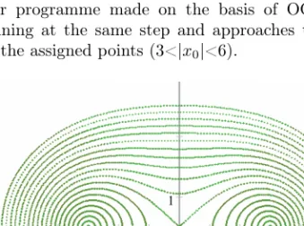
The computer programme made on the basis of OCM assign points along y=0.001 line running at the same step and approaches the points of the curves running through the assigned points (3<|x0|<6).
1 1
Figure 2: This figure was made by using (3.1). The algorithm drew the curves running through the members of the point serial (3<|x0|<6) alongy=0.001 line running at the same step (c=3).
3.2. The approximation of initial values problem by OCM
In the followings we examine how exactly the different algorithms follow the solution. (RKn means thenth-order Runge-Kutta method in the followings.) To the comparison we chose an initial value problem:
y0 = dy dx = 1
2y, y0(0) = 0.005
The y(x) functions giving the solution can not be differentiated in the points where the function and thexaxes intersect. We examined how the applied methods can follow the changes of the curve if we give the starting point in the surroundings of such a point (see Figure 3).
Through the experiment, the initial value of d was 0.005 in the programme which was made on the basis of the OCM.
RK2
RK3
RK4
OCM
1 1
RK2 RK3 RK4
OCM
1 1
RK2 RK3 RK4 OCM
1 h=0.07272395
h=0.05
h=0.025
Figure 3: Where his the step-size of Runge-Kutta algorithms.
Naturally, we can not ignore the fact, that the algorithm based on OCM changes the value ofd in the function of curvature,(which depends on radius of curvature), while the step-size is a constant in RK2, RK3 and RK4.
For the next practical examination of the algorithm we chose the following
ofx-coordinates is different we chose its mean as the step-size of RK algorithms.
RK2
RK3 OCM
1 1
1 1
1 1
Figure 4
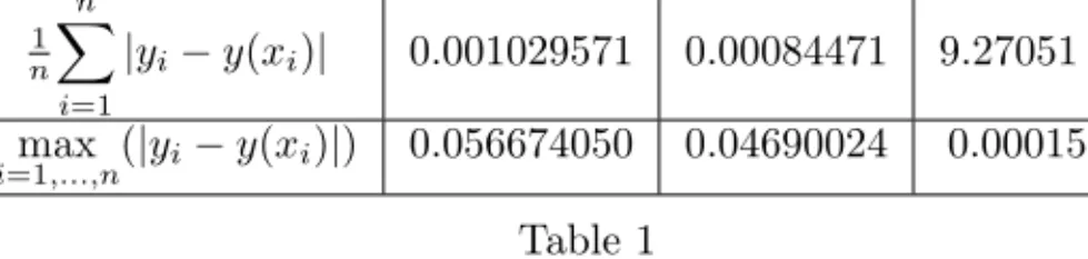
The promptness of approximations was characterised by the average and max- imum of the series of the differences between approximated and calculated values of function (see Table 1).
The graph shows the difference between the calculated value and the values produced by the three procedures in [0;4]. We left out the last two points of 56 points for the sake of better visibility in all three diagrams.
It can be observed that the difference between the approximated values and the calculated ones is increasing in all three cases approaching the zero. It is worth observing and comparing the values belonging to the points showed. It can be seen the last values belonging to RK3 and OCM are almost the same. The figure
RK2 RK3 OCM
1 n
Xn i=1
|yi−y(xi)| 0.001029571 0.00084471 9.27051 10−6
i=1,...,nmax (|yi−y(xi)|) 0.056674050 0.04690024 0.000151908 Table 1
shows that points belonging to RK2 and RK3 are farther from the point where the function and the X-axis cross each other.
Figure 5: We can see that OCM at the same number of steps differs less and better approaches the critical point.
4. Conclusion
It could be seen that with the help of figures produced by a programme operat- ing on the base of OCM we can receive a graphic image about the route of curves running through an assigned points of a domain. Not to mention the fact we can get an image about the route of a curve compared to other curves because this procedure follows the route of curves running through given points. We must not
approximating point. At the same time it needs more calculation and it can be used efficiently in the case when the calculation need of f(x, y) given in (1.1) is high enough.
To receive a clear picture of the promptness of OCM further observations are needed though which it should be compared to other methods using adaptive step- size.
At the same time we can see further possibilities to refine this method.
References
[1] Geda, G., Solving Initial Value Problem by Approximation in Different Graphic Ways,5th Intrnational Conference of PhD Students, Miskolc(2005).
[2] Stoyan, G., Tako, G.,Numerikus módszerek,ELTE-TypoTEX, Budapest, (1993).
[3] Hatvani, L., Pintér, L., Differenciálegyenletes modellek a középiskolában,POLY- GON, Szeged, (1997).
[4] Rontó, M., Raisz, Péterné., Differenciálegyenletek műszakiaknak, Miskolci Egyetemi Kiadó, Miskolc, (2004).
[5] Szőkefalvi-Nagy Gy., Gehér L., Nagy P., Differenciálgeometria, Műszaki Könyvkiadó, Budapest,, (1979).
[6] Geda, G.,Kezdeiérték-probléma közelítő megoldásának egy geometriai szemléltetése, Tavaszi Szél, Debrecen, (2005).
[7] Pólya, Gy.,Matematikai módszerek a természettudományban,Gondolat, Budapest, (1984).
Gábor Geda
Department of Computer Science Eszterházy Károly College Leányka str. 6.
H-3300 Eger, Hungary