123
SPRINGER BRIEFS IN OPTIMIZATION
Balázs Bánhelyi Tibor Csendes Balázs Lévai László Pál
Dániel Zombori
The GLOBAL Optimization Algorithm
Newly Updated with
Java Implementation
and Parallelization
SpringerBriefs in Optimization
Series Editors Sergiy Butenko Mirjam D¨ur Panos M. Pardalos J´anos D. Pint´er Stephen M. Robinson Tam´as Terlaky My T. Thai
SpringerBriefs in Optimization showcases algorithmic and theoretical tech- niques, case studies, and applications within the broad-based field of optimization.
Manuscripts related to the ever-growing applications of optimization in applied mathematics, engineering, medicine, economics, and other applied sciences are encouraged.
More information about this series athttp://www.springer.com/series/8918
Bal´azs B´anhelyi
•Tibor Csendes
•Bal´azs L´evai L´aszl´o P´al
•D´aniel Zombori
The GLOBAL Optimization Algorithm
Newly Updated with Java Implementation and Parallelization
123
Bal´azs B´anhelyi
Department of Computational Optimization University of Szeged
Szeged, Hungary Bal´azs L´evai NNG Inc Szeged, Hungary D´aniel Zombori
Department of Computational Optimization University of Szeged
Szeged, Hungary
Tibor Csendes
Department of Computational Optimization University of Szeged
Szeged, Hungary L´aszl´o P´al
Sapientia Hungarian University of Transylvania
Miercurea Ciuc Romania
ISSN 2190-8354 ISSN 2191-575X (electronic) SpringerBriefs in Optimization
ISBN 978-3-030-02374-4 ISBN 978-3-030-02375-1 (eBook) https://doi.org/10.1007/978-3-030-02375-1
Library of Congress Control Number: 2018961407 Mathematics Subject Classification: 90-08, 90C26, 90C30
© The Author(s), under exclusive licence to Springer International Publishing AG, part of Springer Nature 2018
This work is subject to copyright. All rights are reserved by the Publisher, whether the whole or part of the material is concerned, specifically the rights of translation, reprinting, reuse of illustrations, recitation, broadcasting, reproduction on microfilms or in any other physical way, and transmission or information storage and retrieval, electronic adaptation, computer software, or by similar or dissimilar methodology now known or hereafter developed.
The use of general descriptive names, registered names, trademarks, service marks, etc. in this publication does not imply, even in the absence of a specific statement, that such names are exempt from the relevant protective laws and regulations and therefore free for general use.
The publisher, the authors and the editors are safe to assume that the advice and information in this book are believed to be true and accurate at the date of publication. Neither the publisher nor the authors or the editors give a warranty, express or implied, with respect to the material contained herein or for any errors or omissions that may have been made. The publisher remains neutral with regard to jurisdictional claims in published maps and institutional affiliations.
This Springer imprint is published by the registered company Springer Nature Switzerland AG The registered company address is: Gewerbestrasse 11, 6330 Cham, Switzerland
Acknowledgments
The authors are grateful to their families for the patience and support that helped to produce the present volume.
This research was supported by the project “Integrated program for training new generation of scientists in the fields of computer science,” EFOP-3.6.3-VEKOP-16- 2017-0002. The project has been supported by the European Union, co-funded by the European Social Fund, and by the J´anos Bolyai Research Scholarship of the Hungarian Academy of Sciences.
v
Contents
1 Introduction. . . 1
1.1 Introduction . . . 1
1.2 Problem Domain. . . 2
1.3 The GLOBAL Algorithm. . . 2
2 Local Search . . . 7
2.1 Introduction . . . 7
2.2 Local Search Algorithms . . . 8
2.2.1 Derivative-Free Local Search . . . 8
2.2.2 The Basic UNIRANDI Method . . . 9
2.2.3 The New UNIRANDI Algorithm. . . 9
2.2.4 Reference Algorithms . . . 14
2.3 Computational Investigations. . . 15
2.3.1 Experimental Settings . . . 15
2.3.2 Comparison of the Two UNIRANDI Versions . . . 16
2.3.3 Comparison with Other Algorithms. . . 18
2.3.4 Error Analysis. . . 19
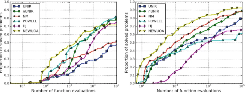
2.3.5 Performance Profiles . . . 22
2.4 Conclusions . . . 25
3 The GLOBALJ Framework. . . 27
3.1 Introduction . . . 27
3.2 Switching from MATLAB to JAVA. . . 28
3.3 Modularization . . . 28
3.4 Algorithmic Improvements . . . 31
3.5 Results . . . 37
3.6 Conclusions . . . 39
vii
viii Contents
4 Parallelization. . . 41
4.1 Introduction . . . 41
4.2 Parallel Techniques. . . 42
4.2.1 Principles of Parallel Computation. . . 42
4.3 Design of PGLOBAL Based on GLOBAL. . . 44
4.4 Implementation of the PGlobal Algorithm. . . 48
4.4.1 SerializedGlobal. . . 48
4.4.2 SerializedClusterizer . . . 51
4.5 Parallelized Local Search. . . 56
4.6 Losses Caused by Parallelization. . . 56
4.7 Algorithm Parameters. . . 56
4.8 Results . . . 57
4.8.1 Environment . . . 57
4.8.2 SerializedGlobal Parallelization Test. . . 58
4.8.3 SerializedGlobalSingleLinkageClusterizer Parallelization Test. . . 61
4.8.4 Comparison of Global and PGlobal Implementations . . . 62
4.9 Conclusions . . . 66
5 Example . . . 69
5.1 Environment. . . 69
5.2 Objective Function . . . 69
5.3 Optimizer Setup. . . 71
5.4 Run the Optimizer. . . 72
5.5 Constraints. . . 73
5.6 Custom Module Implementation. . . 77
A User’s Guide. . . 81
A.1 Global Module. . . 81
A.1.1 Parameters. . . 81
A.2 SerializedGlobal Module . . . 82
A.2.1 Parameters. . . 82
A.3 GlobalSingleLinkageClusterizer Module. . . 83
A.3.1 Parameters. . . 83
A.4 SerializedGlobalSingleLinkageClusterizer Module. . . 84
A.4.1 Parameters. . . 84
A.5 UNIRANDI Module. . . 84
A.5.1 Parameters. . . 84
A.6 NUnirandi Module . . . 85
A.6.1 Parameters. . . 85
A.7 UnirandiCLS Module. . . 85
A.7.1 Parameters. . . 86
A.8 NUnirandiCLS Module . . . 86
A.8.1 Parameters. . . 86
Contents ix
A.9 Rosenbrock Module . . . 87
A.9.1 Parameters. . . 87
A.10 LineSearchImpl Module. . . 87
B Test Functions . . . 89
C DiscreteClimber Code . . . 101
References. . . 107
Chapter 1
Introduction
1.1 Introduction
In our modern days, working on global optimization [25,27,34,38,51,67] is not the privilege of academics anymore, these problems surround us, they are present in our daily life through the increasing number of smart devices to mention one of the most obvious evidences, but they also affect our life when public transport or shipping routes are determined, or the placement of new disposal sites are decided, to come up with some less obvious examples.
Although there are still a lot of open problems in classic mathematical fields [3], like circle packing or covering (e.g., [39,68]), dynamical systems [5,13,14], the list of natural [2], life [4,42,41], and engineering fields of science, which yield new and new problems to solve, is practically infinite. Simultaneously, a good optimization tool becomes more and more valuable especially if it is flexible and capable of addressing a wide range of problems.
GLOBAL is a stochastic algorithm [12,15] aiming to solve bound constrained, nonlinear, global optimization problems. It was the first available implementation of the stochastic global optimization algorithm of Boender et al. [11], which at- tracted several publications in those years and later [6,7,8,9,10,37,53,59,60].
Although, it was competitive and efficient compared to other algorithms, it has not been improved much in the last decade. Its latest implementations were available in FORTRAN, C, and Matlab. Knowing its potential (its competitiveness was doc- umented recently in [15]), we decided to modernize this algorithm to provide the scientific community a whole framework that offers easy customization with more options and better performance than its predecessors.
© The Author(s), under exclusive licence to Springer International Publishing AG, part of Springer Nature 2018
B. B´anhelyi et al.,The GLOBAL Optimization Algorithm,
SpringerBriefs in Optimization,https://doi.org/10.1007/978-3-030-02375-1 1
1
2 1 Introduction
1.2 Problem Domain
In this book, we focus on constrained, nonlinear optimization. Formally, we consider the following global minimization problems:
minxf(x), hi(x) =0 i∈E gj(x)≤0 j∈I
a≤x≤b,
where we search for to the global minimizer point of f, ann-dimensional, real func- tion. The equality and inequality constraint functionshi andgj and the lower and upper boundsaandbof then-dimensional variable vectors determine the feasible set of points. If the constraints are present, we optimize over a new objective func- tion, denoted byF, having the same optimum points as the original function, but it represents the constraints by penalty terms. These increasingly add more and more to the value of f as the point that we evaluateF gets farther and farther from the feasible set of points (for details see [65]). This function replacement results in a much simpler problem:
a≤x≤bmin F(x).
The violation of the upper and lower bounds can easily be avoided if candidate extremal points are generated within the allowed interval during the optimization.
1.3 The GLOBAL Algorithm
GLOBAL is a stochastic, multistart type algorithm that uses clustering to increase efficiency. Stochastic algorithms assume that the problem to be solved is not hope- less in the sense that the relative size of the region of attraction of the global min- imizer points is not too small, i.e., we have a chance to find a starting point in these regions of attraction that can then be improved by a good local search method.
Anyway, if you use a stochastic algorithm, then running it many times may result in different results. Also, it is important to set the sampling density with care to achieve good level of reliability while keeping speed. The theoretical framework of stochastic global optimization methods is described in respective monographs such as [63,74]. The specific theoretical results valid for the GLOBAL algorithm are given in the papers [7,8,11,59,60]. Among others, these state that the expected number of local searches is finite with probability one even if the sampling goes for ever.
Deterministic global optimization methods have the advantage of sure answers compared to the uncertain nature of the results of stochastic techniques (cf. [27,72]).
1.3 The GLOBAL Algorithm 3 On the other hand, deterministic methods [66] are usually more sensitive for the di- mension of the problem, while stochastic methods can cope with larger dimensional ones. The clustering as a tool for achieving efficiency in terms of the number of local searches was introduced by Aimo T¨orn [71].
Algorithm 1.1GLOBAL Input
F:Rn→R
a,b∈Rn: lower and upper bounds Return value
opt∈Rn: a global minimum candidate 1: i←1,N←100,λ←0.5,opt←∞ 2: new,unclustered,reduced,clustered← {}
3: whilestopping criteriaisfalsedo
4: new←new∪generateNsamplefrom[a,b]distributeduni f ormly 5: merged←sortclustered∪newbyascendingorder regardingF 6: last←i·N·λ
7: reduced←select[0,...,last]elementfrommerged 8: x∗←select[0]elementfromreduced
9: opt←minimumof{opt,x∗}
10: clustered,unclustered←clusterreduced 11: new← {}
12: while sizeofunclustered>0do 13: x←popfromunclustered
14: x∗←local searchoverFfromxwithin[a,b] 15: opt←minimumof{opt,x∗}
16: clusterx∗
17: ifx∗isnot clusteredthen 18: create clusterfrom{x∗,x}
19: end if
20: end while 21: i←i+1 22: end while 23: return opt
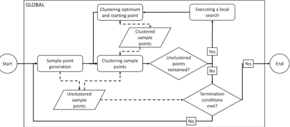
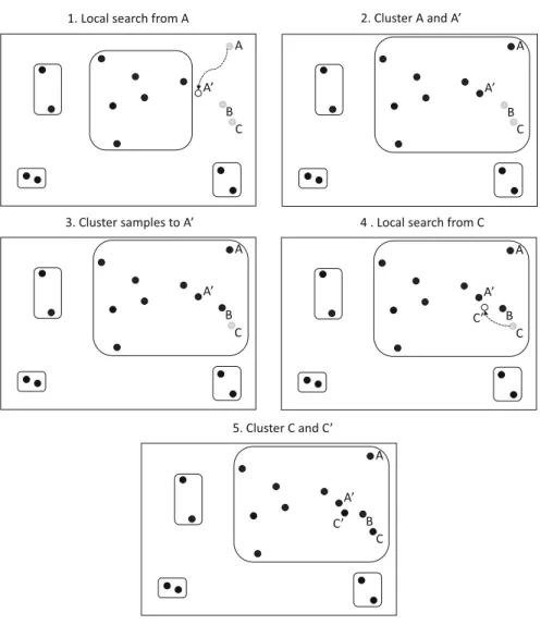
Generally, global optimization is a continuous, iterative production of possible optimizer points until some stopping condition is met. The GLOBAL algorithm creates candidate solutions in two different ways. First, it generates random samples within the given problem space. Second, it starts local searches from promising sample points that may lead to new local optima.
If multiple, different local searches lead to the same local minima, then we gained just confirmation. According to the other viewpoint, we executed unnecessary or, in other words, redundant computation. This happens when many starting points are in the same region of attraction. In this context, the region of attraction of a local minimumx∗is the set of points from which the local search will lead to x∗. With
4 1 Introduction precaution, this inefficiency is reducible if we try to figure out which points are in the same region of attraction. GLOBAL achieves this through clustering.
Before any local search could take place, the algorithm executes a clustering step with the intent to provide information about the possible region of attractions of newly generated samples. Points being in the same cluster are considered as they belong to the same region of attraction. Relying on this knowledge, GLOBAL starts local searches only from unclustered samples, points which cannot be assigned to already found clusters based on the applied clustering criteria. These points might lead us to currently unknown and possibly better local optima than what we already know. The clustering is not definitive in the sense that local searches from unclus- tered points can lead to already found optima, and points assigned to the same clus- ter can actually belong to different regions of attraction. It is a heuristic procedure.
After discussing the motivation and ideas behind, let us have a look over the al- gorithm at the highest level of abstraction (see the pseudo code of Algorithm1.1).
There are two fundamental variables besidei: the loop counter, which areN, the sampling size, andλ, the reduction ratio that modifies the extent of how many sam- ples are carried over into the next iteration. These are tuning parameters to control the extent of memory usage.
The random samples are generated uniformly with respect to the lower and upper bound vectors ofaandb. Upon sample creation and local searching, variables are scaled to the interval[−1,1]nto facilitate computations, and samples are scaled back to the original problem space only when we evaluate the objective function.
A modified single-linkage clustering method tailored to the special needs of the algorithm is responsible for all clustering operations. The original single-linkage clustering is an agglomerative, hierarchical concept. It starts from considering every sample a cluster on its own, then it iteratively joins the two clusters having the closest pair of elements in each round. This criterion is local; it does not take into account the overall shape and characteristics of the clusters; only the distance of their closest members matters.
The GLOBAL single-linkage interpretation follows this line of thought. An un- clustered pointxis added to the first cluster that has a point with a lower objective function than whatxhas, and it is at least as close toxas a predefined critical dis- tancedcdetermined by the formula
dc=
1−αN1−1
1 n,
wherenis the dimension ofFand 0<α<1 is a parameter of the clustering proce- dure. The distance is measured by the infinity norm instead of the Euclidean norm.
You can observe thatdcis adaptive meaning that it becomes smaller and smaller as more and more samples are generated.
The latest available version of GLOBAL applies local solvers for either differen- tiable or non-differentiable problems. FMINCON is a built-in routine of MATLAB using sequential quadratic programming that relies on the BFGS formula when up- dating the Hessian of the Lagrangian. SQLNP is a gradient-based method capable of solving linearly constrained problems using LP and SQP techniques. For non-
1.3 The GLOBAL Algorithm 5 differentiable cases, GLOBAL provides UNIRANDI, a random walk type method.
We are going to discuss this stochastic algorithm in detail later along our improve- ments and proposals. For the line search made in UNIRANDI, one could also apply stochastic process models, also called Bayesian algorithm [40].
The original algorithm proposed by Boender et al. [11] stops if in one main it- eration cycle no new local minimum point is detected. This reflects the assumption that the algorithm parameters are set in such a way that during one such main iter- ation cycle, the combination of sampling, local search, and clustering is capable to identify the best local minimizer points. In other words, the sample size, sample re- duction degree, and critical distance for clustering must be determined in such a way that most of the local minima could be identified within one main iteration cycle.
Usually, some experience is needed to give suitable algorithm parameters. The exe- cution example details in Chapter5and especially those in Section5.3will help the interested reader. Beyond this, some general criteria of termination, like exhausting the allowed number of function evaluations, iterations, or CPU time can be set to stop if it found a given number of local optima or executed a given number of local searches.
Global can be set to terminate if any combination of the classic stopping rules holds true:
1. the maximal number of local minima reached, 2. the allowed number of local searches reached, 3. the maximal number of iterations reached,
4. the maximal number of function evaluations reached, or 5. the allowed amount of CPU time used.
The program to be introduced in the present volume can be downloaded from the address:
http://www.inf.u-szeged.hu/global/
Chapter 2
Local Search
2.1 Introduction
The GLOBAL method is characterized by a global and a local phase. It starts a lo- cal search from a well-chosen initial point, and then the returned point is saved and maintained by the GLOBAL method. Furthermore, there are no limitations regard- ing the features of the objective functions; hence an arbitrary local search method can be attached to GLOBAL. Basically, the local step is a completely separate mod- ule from the other parts of the algorithm. Usually, two types of local search are con- sidered: methods which rely on derivative information and those which are based only on function evaluations. The latter group is also called direct search methods [63]. Naturally, the performance of GLOBAL on a problem depends a lot on the applied local search algorithm. As there are many local search methods, it is not an easy task to choose the proper one.
Originally [12], GLOBAL was equipped with two local search methods: a quasi- Newton procedure with the Davidon-Fletcher-Powell (DFP) update formula [19]
and a direct search method called UNIRANDI [29]. The quasi-Newton local search method is suitable for problems having continuous derivatives, while the random walk type UNIRANDI is preferable for non-smooth problems.
In [15], a MATLAB version of the GLOBAL method was presented with im- proved local search methods. The DFP local search algorithm was replaced by the better performing BFGS (Broyden-Fletcher-Goldfarb-Shanno) variant. The UNI- RANDI procedure was improved so that the search direction was selected by using normal distribution random numbers instead of uniform distribution ones. As a re- sult, GLOBAL become more reliable and efficient than the old version.
© The Author(s), under exclusive licence to Springer International Publishing AG, part of Springer Nature 2018
B. B´anhelyi et al.,The GLOBAL Optimization Algorithm,
SpringerBriefs in Optimization,https://doi.org/10.1007/978-3-030-02375-1 2
7
8 2 Local Search GLOBAL was compared with well-known algorithms from the field of global optimization within the framework of BBOB 2009.1 BBOB 2009 was a con- test of global optimization algorithms, and its aim was to quantify and com- pare the performance of optimization algorithms in the COCO2framework. Now, GLOBAL was equipped withfminunc, a quasi-Newton local search method of MATLAB and with the Nelder-Mead [46] simplex method implemented as in [36].
GLOBAL performed well on ill-conditioned functions and on multimodal weakly structured functions. These aspects were also mentioned in [24], where GLOBAL was ranked together with NEWUOA [55] and MCS [28] as best for a function evaluation budget of up to 500nfunction values. The detailed results can be found in [50].
One of the main features of the UNIRANDI method is its reliability, although the algorithm may fail if the problem is characterized by long narrow valleys or the problem is ill-conditioned. This aspect is more pronounced as the dimension grows.
Recently we investigated an improved variant of the UNIRANDI method [48,49]
and compared it with other local search algorithms.
Our aim now is to confirm the efficiency and reliability of the improved UNI- RANDI method by including in the comparisons of other well-known derivative- free local search algorithms.
2.2 Local Search Algorithms 2.2.1 Derivative-Free Local Search
Derivative-free optimization is an important branch of the optimization where usu- ally no restrictions are applied to the optimization method regarding the derivative information. Recently a growing interest can be observed to this topic from the scientific community. The reason is that many practical optimization problems can only be investigated with derivative-free algorithms. On the other hand with the in- creasing capacity of the computers and with the available parallelization techniques, these problems can be treated efficiently.
In this chapter, we consider derivative-free local search methods. They may be- long to two main groups: direct search methods and model-based algorithms. The first group consists of methods like the simplex method [46], coordinate search [54], and pattern search, while in the second group belong trust-region type methods like NEWUOA [55]. The reader can find descriptions of most of these methods in [61].
1http://www.sigevo.org/gecco-2009/workshops.html#bbob.
2http://coco.gforge.inria.fr.
2.2 Local Search Algorithms 9
2.2.2 The Basic UNIRANDI Method
UNIRANDI is a very simple, random walk type local search method, originally proposed by J¨arvi [29] at the beginning of the 1970s and later used by A.A. T¨orn in [71]. UNIRANDI was used together with the DFP formula as part of a clus- tering global optimization algorithm proposed by Boender et al. [11]. Boender’s algorithm was modified in several points by Csendes [12], and with the two lo- cal search methods (UNIRANDI and DFP), the algorithm was implemented called GLOBAL.
UNIRANDI relies only on function evaluations and hence can be applied to problems where the derivatives don’t exist or they are expensive to evaluate. The method has two main components: the trial direction generation procedure and the line search step. These two steps are executed iteratively until some stopping condi- tion is met.
Algorithm 2.1 shows the pseudocode of the basic UNIRANDI local search method. The trial point computation is based on the current starting point, on the generated random direction (d), and on the step length parameter (h). The parame- terhhas a key role in UNIRANDI since it’s value is adaptively changed depending on the successful or unsuccessful steps. The opposite direction is tried if the best function value can’t be reduced along the current direction (line 11). The value of the step length is halved if none of the two directions were successful (line 19).
A discrete line search (Algorithm 2.2) is started if the current trial point de- creases the best function value. It tries to achieve further function reduction along the current direction by doubling the actual value of step length huntil no more reduction can be achieved. The best point and the actual value of the step length are returned.
2.2.3 The New UNIRANDI Algorithm
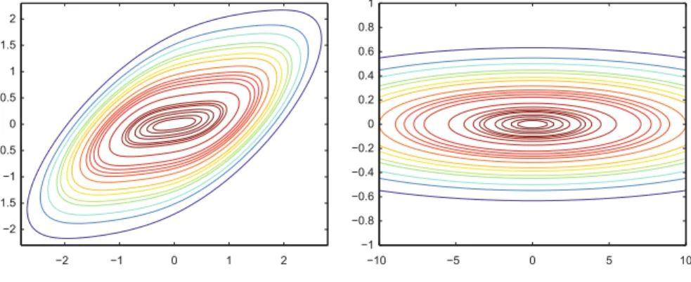
One drawback of the UNIRANDI method is that it performs poorly on ill- conditioned problems. This kind of problems is characterized by long, almost par- allel contour lines (see Figure2.1); hence function reduction can only be achieved along hard-to-find directions. Due to the randomness of the UNIRANDI local search method, it is even harder to find good directions in larger dimensions. As many real-world optimization problems have this feature of ill-conditioning, it is worth to improve the UNIRANDI method to cope successfully with this type of problems.
10 2 Local Search Algorithm 2.1The basic UNIRANDI local search method
Input
f- the objective function x0- the starting point
tol- the threshold value of the step length Return value
xbest,fbest- the best solution found and its function value 1: h←0.001
2: f ails←0 3: xbest←x0
4: whileconvergence criterion is not satisfieddo 5: d∼N(0,III)
6: xtrial←xbest+h·d 7: iff(xtrial)<f(xbest)then
8: [xbest,fbest,h]←LineSearch(f,xtrial,xbest,d,h) 9: h←0.5·h
10: else
11: d← −d
12: xtrial←xbest+h·d
13: iff(xtrial)<f(xbest)then
14: [xbest,fbest,h]←LineSearch(f,xtrial,xbest,d,h)
15: h←0.5·h
16: else
17: f ails←f ails+1
18: iff ails≥2then
19: h←0.5·h
20: f ails←0
21: ifh<tolthen
22: return
23: end if
24: end if
25: end if
26: end if 27: end while
Coordinate search methods iteratively perform line search along one axis di- rection at the current point. Basically, they are solving iteratively univariate opti- mization problems. Well-known coordinate search algorithms are the Rosenbrock method [63], the Hooke-Jeeves algorithm [26], and Powell’s conjugate directions method [54].
2.2 Local Search Algorithms 11
−2 −1 0 1 2
−2
−1.5
−1
−0.5 0 0.5 1 1.5 2
−10 −5 0 5 10
−1
−0.8
−0.6
−0.4
−0.2 0 0.2 0.4 0.6 0.8 1
Fig. 2.1 Ill-conditioned functions
Algorithm 2.2TheLineSearchfunction Input
f- the objective function xtrial- the current point xbest- the actual best point
dandh- the current direction and step length Return value
xbest,fbest,h- the best point, the corresponding function value, and the step length 1: whilef(xtrial)<f(xbest)do
2: xbest←xtrial
3: fbest←f(xbest) 4: h←2·h
5: xtrial←xbest+h·d 6: end while
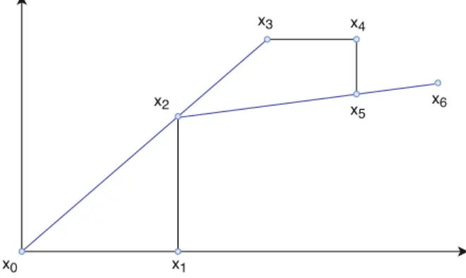
The Rosenbrock method updates in each iteration an orthogonal coordinate sys- tem and makes a search along an axis of it. The Hooke-Jeeves method performs an exploratory search in the direction of coordinate axes and does apattern search (Figure2.2) in other directions. The pattern search is a larger search in the improv- ing direction also calledpattern direction. The Powell’s method tries to discard one direction in each iteration step by replacing it with the pattern direction. One impor- tant feature of these algorithms is that they can follow easily the contour lines of the problems having narrow, turning valley-like shapes.
12 2 Local Search
Fig. 2.2 Pattern search along the directionsx2−x0andx5−x2
Inspired by the previously presented coordinate search methods, we introduced some improvements to the UNIRANDI algorithm. The steps of the new method are listed in Algorithm2.3. The UNIRANDI local search method was modified so that after a given number of successful line searches along random directions (lines 7–36), two more line searches are performed along pattern directions (lines 39–53).
Algorithm 2.3The new UNIRANDI local search algorithm Input
f- the objective function x0- the starting point
tol- the threshold value of the step length Return value
xbest,fbest- the best solution found and its function value 1: h←0.001
2: f ails←0 3: xbest←x0
4: whileconvergence criterion is not satisfieddo 5: itr←0
6: Letdirsi,i=1...maxitersinitialized with the null vector 7: whileitr<maxitersdo
8: d∼N(0,III)
9: xtrial←xbest+h·d
10: iff(xtrial)<f(xbest)then
11: [xbest,fbest,h]←LineSearch(f,xtrial,xbest,d,h)
12: h←0.5·h
13: f ails←0
14: itr←itr+1
15: dirsitr←xbest−x0
16: else
17: d← −d
18: xtrial←xbest+h·d
19: iff(xtrial)<f(xbest)then
2.2 Local Search Algorithms 13 20: [xbest,fbest,h]←LineSearch(f,xtrial,xbest,d,h)
21: h←0.5·h
22: f ails←0
23: itr←itr+1
24: dirsitr←xbest−x0
25: else
26: f ails←f ails+1
27: iff ails≥2then
28: h←0.5·h
29: f ails←0
30: ifh<tolthen
31: return
32: end if
33: end if
34: end if
35: end if
36: end while
37: The best point is saved as the starting point for the next iteration:x0←xbest
38: Letd1←dirsitrandd2←dirsitr−1the last two pattern directions saved during the pre- vious iterations
39: fori∈ {1,2}do
40: xtrial←xbest+h·di
41: iff(xtrial)<f(xbest)then
42: [xbest,fbest,h]←LineSearch(f,xtrial,xbest,di,h)
43: h←0.5·h
44: else
45: di← −di
46: xtrial←xbest+h·di
47: iff(xtrial)<f(xbest)then
48: [xbest,fbest,h]←LineSearch(f,xtrial,xbest,di,h)
49: h←0.5·h
50: end if
51: end if
52: end for 53: end while
After each successful line search, new pattern directions are computed and saved in lines 15 and 24. The role of the f ailsvariable is to follow the unsuccessful line search steps, and the value of thehparameter is halved if two consecutive failures occur (line 27). This step preventshto decrease quickly, hence avoiding a premature exit from the local search algorithm.
In the final part of the algorithm (lines 39–52), pattern searches are performed along the last two pattern directions (dirsitranddirsitr−1) computed during the pre- vious iterations.
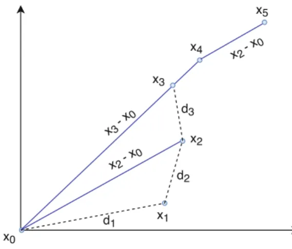
These steps can be followed in two-dimensions on Figure 2.3. After three searches along random directions (d1,d2, andd3), we take two line searches along the pattern directionsx3−x0andx2−x0in order to speed-up the optimization pro- cess.
14 2 Local Search
Fig. 2.3 Improved UNIRANDI: search along pattern directionsx3−x0andx2−x0
2.2.4 Reference Algorithms
The following derivative-free algorithms are considered for comparison in the sub- sequent sections: Nelder-Mead simplex method (NM), Powell’s conjugate gradient method (POWELL), Hooke-Jeeves algorithm (HJ), and NEWUOA, a model-based method.
Nelder-Mead Simplex Method [46] The method uses the concept of a simplex, a set ofn+1 points inndimension. The algorithm evaluates all then+1 points of the simplex and attempts to replace the point with the largest function value with a new candidate point. The new point is obtained by transforming the worst point around the centroid of the remaining n points using the following operations: reflection, expansion, and contraction.
As the shape of the simplex can be arbitrarily flat, it is not possible to prove global convergence to stationary points. The method can stagnate and converge to a non-stationary point. In order to prevent stagnation, Kelley [35] proposed a restarted variant of the method that uses an approximate steepest descent step.
Although the simplex method is rather old, it still belongs to the most reliable algorithms especially in lower dimensions [52]. In this study, we use the implemen- tation from [35].
Powell’s Algorithm [54] It tries to construct a set of conjugate directions by using line searches along the coordinate axes. The method initialize a set of directionsui
to the unit vectorsei,i=1,...,n. A search is started from an initial pointP0by performingnline searches along directionsui. LetPnbe the point found afternline searches. After these steps the algorithm updates the set of directions by eliminating the first one (ui=ui+1,i=1,...,n−1) and setting the last direction toPn−P0. In the last step, one more line search is performed along the directionun.
2.3 Computational Investigations 15 In [43], a recent application of Powell’s method is presented. We used a MAT- LAB implementation of the method described in [56].
Hooke-Jeeves Method [26] It is a pattern search technique which performs two types of search: an exploratory search and a pattern move. The exploratory search is a kind of a neighboring search where the current point is perturbed by small amounts in each of the variable directions. The pattern move is a longer search in the improving direction. The algorithm makes larger and larger moves as long as the improvement continues. We used the MATLAB implementation from [36].
NEWUOA Algorithm [55] NEWUOA is a relatively new local search method for unconstrained optimization problems. In many papers [18,24,61,21], it appeared as a reference algorithm, and it is considered to be a state-of-the-art solver.
The algorithm employs a quadratic approximation of the objective function in the trust region. In each iteration, the quadratic model interpolates the function at 2n+1 points. The remaining degree of freedom is taken up by minimizing the Frobenius norm of the difference between the actual and previous model.
We used the implementation from NLopt [30] through the OPTI TOOLBOX [17]
which offered a MATLAB MEX interface.
2.3 Computational Investigations 2.3.1 Experimental Settings
We have conducted some computational simulations as follows: at first, the im- proved UNIRANDI algorithm (nUNIR) was compared with the previous version (UNIR) in terms of reliability and efficiency. The role of the second experiment is to explore the differences between the new UNIRANDI method and the reference algorithms presented previously. In the third experiment, all the local search meth- ods were tested in terms of error value, while in the final stage, the performance of the methods was measured in terms of percentage of solved problems. During the simulations, the local search methods were tested as a part of the GLOBAL algorithm.
The testbed consists of 63 problems with characteristics like separability, non- separability, and ill-conditioning. For some problems, the rotated and shifted ver- sions were also considered. Thirty-eight of the problems are unimodal, and 25 are multimodal with the dimensions varying between 2 and 60.
The main comparison criteria are the following: the average number of function evaluations (NFE), the success rate (SR), and the CPU time. SR equals to the ratio of the number of successful trials to the total number of trials expressed as a per- centage. A trial is considered successful if|f∗−fbest| ≤10−8 holds, where f∗is the known global minimum value, while fbest is the best function value obtained.
The function evaluations are not counted if a trial fails to find the global minimum;
16 2 Local Search hence it counts as an unsuccessful run. The different comparison criteria are com- puted over 100 independent runs with different random seeds. In order to have a fair comparison, the same random seed was used with each local search algorithm.
The maximal allowed function evaluation budget during a trial was set to 2·104· n. The GLOBAL algorithm runs until it finds the global optimum with the specified precision or when the maximal number of function evaluations is reached. In each iteration of GLOBAL, 50 random points were generated randomly, and the 2 best points were selected for the reduced sample. A local search procedure inside the GLOBAL algorithm stops if it finds the global optimum with the specified precision or the relative function value is smaller than 10−15. They also stop when the number of function evaluations is larger than half of the total available budget.
During the optimization process, we ignored the boundary handling technique of the UNIRANDI method since the other algorithms do not have this feature.
All computational tests have been conducted under MATLAB R2012a on a 3.50 GHz Intel Core i3 machine with 8 Gb of memory.
2.3.2 Comparison of the Two UNIRANDI Versions
In the current subsection, we analyze the reliability and the efficiency of the two versions of the UNIRANDI method. The comparison metrics were based on the average function evaluations, success rate, and CPU time. The corresponding values are listed in Tables2.1and2.2.
The success rate values show that the new UNIRANDI local search method is more reliable than the old one. Usually, the earlier, called nUNIR, has larger or equal SR values than UNIR, except the three multimodal functions (Ackley, Rastrigin, and Schwefel). UNIR fails to converge on ill-conditioned functions like Cigar, Ellipsoid, and Sharpridge but also on problems that have a narrow curved valley structure like Rosenbrock, Powell, and Dixon-Price. The available budget is not enough to find the proper directions on these problems. The SR value of the nUNIR method is almost 100% in most of the cases except some hard multimodal functions like Ackley, Griewank, Perm, Rastrigin, and Schwefel.
Considering the average number of function evaluations, nUNIR requires less number of function evaluations than UNIR, especially on the difficult problems.
nUNIR is much faster on the ill-conditioned problems, and the differences are more pronounced in larger dimensions (e.g., Discus, Sum Squares, and Zakharov). On the problems with many local minima, the nUNIR is again faster than UNIR ex- cept the Ackley, Griewank, and Schwefel functions. The CPU time also reflects the superiority of the nUNIR method over UNIR on most of the problems.
The last line of Tables 2.1and 2.2show the average values of the indicators (NFE, CPU) computed over those problems where at least one trial was successful for both of the methods. The SR is computed over the entire testbed. The aggregated values of NFE, SR, and CPU time again show the superiority of the nUNIR method over UNIR.
2.3 Computational Investigations 17 Table 2.1 Comparison of the two versions of the UNIRANDI method in terms of number of function evaluations (NFE), success rate (SR), and CPU time—part 1
Function UNIR nUNIR
dim NFE SR CPU NFE SR CPU
Ackley 5 25,620 93 0.5479 32,478 87 0.7485
Beale 2 3133 98 0.0353 3096 98 0.0356
Booth 2 168 100 0.0062 185 100 0.0067
Branin 2 172 100 0.0064 170 100 0.0064
Cigar 5 68,357 41 0.5072 542 100 0.0133
Cigar 40 − 0 4.3716 6959 100 0.1140
Cigar-rot 5 57,896 57 0.9968 930 100 0.0317
Cigar-rot 40 − 0 11.9116 16,475 100 0.4034
Cigar-rot 60 − 0 20.3957 28,062 100 0.6363
Colville 4 15,361 100 0.1399 1524 100 0.0226
Diff. Powers 5 − 0 0.7139 1926 100 0.0340
Diff. Powers 40 − 0 9.7129 91,786 100 1.2864
Diff. Powers 60 − 0 18.5559 189,939 100 3.1835
Discus 5 5582 100 0.0555 1807 100 0.0253
Discus 40 23,480 100 0.2309 19,484 100 0.2354
Discus-rot 5 5528 100 0.1342 4477 100 0.1232
Discus-rot 40 23,924 100 0.4317 20,857 100 0.4153 Discus-rot 60 30,910 100 0.5558 27,473 100 0.5196 Dixon-Price 10 74,439 80 0.6853 15,063 100 0.1850
Easom 2 717 100 0.0133 1629 100 0.0295
Ellipsoid 5 41,611 100 0.2998 976 100 0.0170
Ellipsoid 40 − 0 9.7700 44,619 100 0.7159
Ellipsoid-rot 5 41,898 100 0.6076 3719 100 0.1058 Ellipsoid-rot 40 − 0 17.1149 71,799 100 1.7026 Ellipsoid-rot 60 − 0 26.7447 120,476 100 2.9285 Goldstein Price 2 233 100 0.0064 228 100 0.0072
Griewank 5 43,749 34 0.7231 44,944 34 0.7816
Griewank 20 12,765 100 0.1839 11,801 100 0.1792
Hartman 3 878 100 0.0298 241 100 0.0128
Hartman 6 9468 100 0.2168 1056 100 0.0513
Levy 5 31,976 77 0.6050 17,578 99 0.3083
Matyas 2 172 100 0.0062 188 100 0.0069
Perm-(4,1/2) 4 − 0 0.7295 44,112 44 0.7426
Perm-(4,10) 4 5076 1 0.8043 16,917 99 0.2437
Powell 4 43,255 33 0.5409 1787 100 0.0359
Powell 24 − 0 3.5950 42,264 100 0.4767
Power Sum 4 16,931 10 0.7003 33,477 86 0.4677 Rastrigin 4 36,665 22 0.6912 34,449 21 0.7817
Average 20,746 60 0.3247 11,405 95 0.2043
18 2 Local Search Table 2.2 Comparison of the two versions of the UNIRANDI method in terms of number of function evaliations (NFE), success rate (SR), and CPU time—part 2
Function UNIR nUNIR
dim NFE SR CPU NFE SR CPU
Rosenbrock 5 – 0 0.6763 2227 100 0.0415 Rosenbrock 40 – 0 5.7691 70,624 100 0.7062 Rosenbrock-rot 5 – 0 1.5023 1925 100 0.0719 Rosenbrock-rot 40 – 0 12.7113 78,104 100 1.4457 Rosenbrock-rot 60 – 0 20.0845 137,559 100 2.3171 Schaffer 2 18,728 36 0.2469 14,270 94 0.1499 Schwefel 5 57,720 40 0.7215 58,373 37 0.7733 Shekel-5 4 1314 100 0.0488 1401 100 0.0543 Shekel-7 4 1506 100 0.0513 1646 100 0.0616 Shekel-10 4 1631 100 0.0573 1817 100 0.0658
Sharpridge 5 – 0 0.9025 961 100 0.0209
Sharpridge 40 – 0 7.0828 12,755 100 0.2337 Shubert 2 854 100 0.0206 827 100 0.0211 Six hump 2 137 100 0.0058 139 100 0.0070
Sphere 5 292 100 0.0106 331 100 0.0122
Sphere 40 2698 100 0.0682 2799 100 0.0788 Sum Squares 5 373 100 0.0134 396 100 0.0147 Sum Squares 40 21,973 100 0.3337 8205 100 0.1696 Sum Squares 60 49,435 100 0.6189 15,053 100 0.3084 Sum Squares-rot 60 47,700 100 0.8876 17,472 100 0.4365 Trid 10 5588 100 0.0964 2057 100 0.0440 Zakharov 5 427 100 0.0148 465 100 0.0151 Zakharov 40 18,784 100 0.2799 16,913 100 0.2761 Zakharov 60 41,633 100 0.4633 36,191 100 0.4407 Zakharov-rot 60 42,813 100 0.9140 37,799 100 0.8689 Average 20,746 60 0.3247 11,405 95 0.2043
2.3.3 Comparison with Other Algorithms
This subsection presents comparison results between the new UNIRANDI method and the reference algorithms of Nelder-Mead, POWELL, Hooke-Jeeves, and the NEWUOA method. The main indicators of comparison are the average number of function evaluations and success rate. The results are listed in Tables2.3and2.4.
Considering the success rate values, we can observe the superiority of the nUNIR and NEWUOA algorithms over the other methods. The smallest values for nUNIR are shown for some hard multimodal problems like Griewank, Perm, Rastrigin, and Schwefel with 34%, 44%, 21%, and 37%, respectively. NEWOUA has almost 100%
values everywhere; however, it fails on all the trials for the Different Powers (40 and 60 dimensions) and Sharpridge (40 dimension) functions. Although the POWELL and Hooke-Jeeves techniques have similar behavior, the success rate values differ often significantly. The Nelder-Mead simplex method usually fails in the trials in higher dimensions, but in small dimensions, it shows very good values.