on the topic:
“Robot Navigation in Unknown and Dynamic Environment”
by:
Neerendra Kumar
(Ph.D. Student)
Supervisor:
Dr. Zoltán Vámossy
(Associate Professor)
Doctoral School of Applied Informatics and Applied Mathematics
Budapest, 2020
Chair:
Dr. József K. Tar, Full Professor, DSc, ÓE Members:
Dr. Márta Takács, Associate Professor, PhD, ÓE Dr. Szabolcs Sergyán, Associate Professor, PhD
Home Defence Committee:
Opponents:
Dr. József K. Tar, Full Professor, DSc, ÓE Dr. Szilveszter Kovács, Associate Professor, PhD, ME
Public Defence Committee:
Opponents:
Dr. Szilveszter Kovács, Associate Professor, PhD, ME Dr. Márta Takács, Associate Professor, PhD, ÓE
Chair:
Dr. József K. Tar, Full Professor, DSc, ÓE Secretary:
Dr. Sándor Szénási, Associate Professor, PhD, ÓE Second Secretary:
Dr. Adrienn Dineva, Assistant Professor, PhD, ÓE Members:
Dr. Róbert Fullér, Full Professor, DSc, SZE Dr. Szilveszter Pletl, Professor, PhD, SZTE Dr. Edit Laufer, Associate Professor, PhD, ÓE
I, Neerendra Kumar, declare that the thesis entitled, ‘Robot Navigation in Unknown and Dynamic Environment’ and the content presented in it, is entirely my own research work in the able supervision of Dr. Zoltán Vámossy (Associate Professor).
It is hereby assured that:
• This work has been completed as a candidate for PhD degree at Óbuda University.
• Wherever in the thesis the published work of other authors is consulted, this work is clearly referenced.
• Wherever in the thesis quotations from other authors are used, then this fact is clearly mentioned. The thesis is absolutely my own work with the exception of such quotations.
• All the main sources of help have been properly acknowledged .
Budapest . . . .
September 3, 2020. Neerendra Kumar
(PhD Candidate)
General Hannibal Barca
Above all, I am extremely grateful to my Ph.D. supervisor,Dr. Zoltán Vámossy, for his continuous expert guidance, support and motivation during my Ph.D. research work.
He always responded my queries, emails and paper corrections very quickly. Further, my supervisor, always supported me, promptly, about the document requirements of the Universities pertaining to this study. I have always got positive response from him for our meetings to discuss the research problems and the possible solutions.
I am greatly thankful to Prof. Aurél Galántai, the head of the Doctoral School of Applied Informatics and Applied Mathematicsof the Óbuda University, for his immense support and leadership to improve the results and to achieve the final goal of the work.
I am highly thankful to Prof. László Horváth for his valuable and motivational comments on my oral presentations of end semester research reports and on my research paper presentations in various internal conferences. I am grateful to Prof. Levente Kovácsfor his interesting and easy to grasp subject lectures and his continuous inspiration to attend the international conferences related to my work. From bottom of my heart, I am thankful toProf. József K. Tar for his knowledgeable subject lectures and his provocation to use open source software.
I am wholeheartedly thankful to Mr. Zsolt Miklós Szabó-Resch for providing me his technical expertise and guidance onLinux, robot operating system, Gazebo simulator and robot handling. My profound thanks to Dr. György Eigner for sharing the important information related Ph.D. degree procedure and formats of required documents and research reports. My sincere thanks toMs. Zsuzsanna BácskaiandMs. Katalin Hersicsfor their administrative support throughout my study atÓbuda University.
I am greatly thankful to the governments of Hungary and India for selecting me for the Tempus Public Foundation’s prestigious Stipendium Hungaricum Scholarship Programme to get admission in this Ph.D. programme.
A lot of thanks to Prof. Ashok Aima, Vice Chancellor of Central University of Jammu, India, for granting me the study leave to pursue this Ph.D. study. I am grateful to Prof. Lokesh Verma, Prof. Devanand and my fellow colleagues of Central University of Jammu for their support in the study leave.
I would also like to thank to all of those who are not namely listed here, like, my professors, many of my friends and colleagues from whom I got inspired and learnt a lot.
Finally, I give my heartily thanks to my loving family members for their support.
This dissertation presents the research work carried out on robot navigation. The introductionand theconclusionof the study are provided in Chapters1and6, respectively.
Chapter2presents scientific methods applied in the research work. Chapter3is dedicated to the robot navigation in known and static environment. The robot navigation in unknown and dynamic environment has been considered in Chapter 4. In Chapter 5, advanced algorithms are proposed for the obstacle recognition and obstacle avoidance in unknown and static environments.
The dissertation has covered the robot-navigation-problem in the three main categories of the environments in which the robot may navigate.
Firstly, the robot navigation in known and static environment is considered in Chapter 3. In Chapter3, the A* algorithm is implemented in the global path planner of the robot.
The result obtained from the different heuristic functions has been compared. Further, theProbabilistic Roadmaps (PRM)technique is used to find an obstacle-free-path from start to goal.
Secondly, the robot navigation in unknown and dynamic environment is taken into consideration in Chapter4. In Chapter 4, an algorithm for obstacle avoidance has been evolved using the bumper hit events of the robot. Further, robot navigation models are presented using MATLAB-Simulink. The robot navigation models use fuzzy controllers for obstacle avoidance during robot navigation. For the fuzzy controllers, appropriate Fuzzy Inference Systems (FISs) are developed and implemented by using Mamdani and Sugeno types ofFISs.
Thirdly, the robot navigation in unknown and static environment is presented in Chapter5. In Chapter 5, the main results are presented by a theses group. The theses group contains three thesis points (5.4.1−5.4.3). The thesis point in5.4.1 is based on the proposed algorithm for obstacle recognition. The thesis point5.4.2 is obtained from the proposed advanced algorithm possessing obstacle recognition and obstacle avoidance features. Finally, the “two sample t-test” is applied, for obstacle recognition and avoidance in robot navigation, to present the thesis point5.4.3.
The newly proposed concepts, methods and algorithms are tested on simulatedTurtlebot robot in Gazebo simulator. The experimental results for the real Turtlebot robot has also been included wherever it was possible. As background information, the related appendices are provided at the end of the dissertation.
Acronyms xxi
1. Introduction 1
1.1. Background of the research . . . 1
1.1.1. Research gaps in the existing solutions . . . 6
1.2. Dissertation outline. . . 6
2. Hardware, software, and scientific methods applied in the research work 8 2.1. Hardware and software used for experimental set-up . . . 8
2.2. Mathematical foundations of applied soft computing techniques . . . 9
2.2.1. Artificial neural network (ANN) . . . 9
2.2.2. Fuzzy logic . . . 10
2.2.2.1. Fuzzy set . . . 10
2.2.2.2. Membership functions . . . 11
2.2.3. Fuzzy inference system. . . 14
2.2.3.1. Fuzzification . . . 15
2.2.3.2. Defuzzification . . . 15
2.2.4. Adaptive neuro-fuzzy inference system (ANFIS) . . . 16
3. Robot navigation with obstacle avoidance in known and static environment 19 3.1. Heuristic approaches in robot navigation . . . 19
3.1.1. A* algorithm and the heuristic functions. . . 19
3.1.2. Implementation and experimental results . . . 20
3.1.3. Summary . . . 24
3.2. Robot path pursuit using probabilistic roadmaps . . . 25
3.2.1. Preliminary work . . . 25
3.2.1.1. Extracting optimal way-points from the environment . . 25
3.2.1.2. Occupancy grid map of the environment . . . 26
3.2.2. Probabilistic roadmaps. . . 28
3.2.3. Path pursuit . . . 30
3.2.4. Summary . . . 31
4. Robot navigation with obstacle avoidance in unknown and dynamic environ- ment 32 4.1. Robot obstacle avoidance using bumper event . . . 32
4.1.1. Bumper-event based algorithm . . . 32
4.1.2. Implementation and experimental results . . . 33
4.1.3. Summary . . . 36
4.2. Robot navigation in unknown environment using fuzzy logic . . . 37
4.2.1. LASER scan data for obstacle avoidance. . . 38
4.2.2. The fuzzy controller . . . 39
4.2.2.1. Fuzzy logic design . . . 39
4.2.2.2. Membership functions . . . 41
4.2.2.3. Fuzzy rule base. . . 43
4.2.3. Implementation of the model in MATLAB–Simulink . . . 44
4.2.4. Experimental set-up and results . . . 46
4.2.5. Summary . . . 48
4.3. Robot navigation with obstacle avoidance in unknown environment using adaptive neuro-fuzzy inference system . . . 49
4.3.1. Robot navigation model in MATLAB-Simulink . . . 49
4.3.2. Sugeno-type FIS for the Fuzzy Controller . . . 52
4.3.3. Results . . . 55
4.3.4. Summary . . . 57
5. Obstacle recognition and avoidance during robot navigation in unknown static environment 59 5.1. Robot navigation with obstacle recognition using LASER sensor . . . 59
5.1.1. Problem definition and solution . . . 60
5.1.2. Experimental results and discussion . . . 62
5.1.3. Summary . . . 67
5.2. Obstacle recognition and avoidance during robot navigation in unknown static environment . . . 68
5.2.1. Robot navigation model and problem definition . . . 68
5.2.2. Advanced algorithm for obstacle avoidance with obstacle recognition 72 5.2.3. Experimental results . . . 74
5.2.4. Summary . . . 76
5.3. Obstacle recognition and avoidance using two-sample t-test . . . 77
5.3.1. The Student’s t . . . 77
5.3.2. t-Test for single mean . . . 78
5.3.3. t-Test for difference of two means. . . 78
5.3.4. Obstacle recognition and avoidance using t-test . . . 79
5.3.5. Experimental results and discussion . . . 80
5.3.6. Summary . . . 81
5.4. Theses group: Robot navigation with obstacle recognition in unknown static environment having rectangular obstacles. . . 82
5.4.1. Thesis point-Robot navigation in unknown static environment with obstacle recognition using LASER sensor . . . 82
5.4.2. Thesis point-Obstacle recognition and avoidance during robot navi- gation in unknown static environment . . . 82
5.4.3. Thesis point-Application of t-test for obstacle recognition and avoid- ance in robot navigation . . . 82
6. Conclusion, applicability, and future research scope 83 6.1. Conclusion . . . 83
6.2. Applicability of the results and future research scope . . . 84
Bibliography 85 A. Appendices 100 A.1. Simulated Turtlebot robot in Gazebo simulator . . . 100
A.1.1. Creating user-defined Gazebo-world . . . 100
A.1.2. Pre-defined Gazebo-worlds in turtlebot_gazebo package . . . 100
A.2. Communication between software packages using ROS . . . 101
A.3. Pre-defined and user-defined ROS nodes . . . 103
A.4. Graphical representation and execution of ROS nodes . . . 103
A.4.1. Executing user-defined node with simulated robot . . . 105
A.4.2. Executing user-defined node with real robot . . . 106
A.5. Map of the navigation environment . . . 106
A.5.1. Building map of the environment using ROS package. . . 106
A.5.2. Turtlebot’s autonomous navigation with given map . . . 107
A.5.3. Creating user-defined global planner . . . 108
A.6. Writing robot positions in a text file . . . 109
A.7. Creating occupancy grid map using MATLAB. . . 110
A.8. Generating probabilistic roadmaps in MATLAB. . . 111 A.9. Critical values of t for t-test . . . 111
1.1. Structure of the dissertation. . . 7
2.1. Artificial neuron model given by [81]. . . 9
2.2. Triangle Membership Function (MF) having support and core as [2,7] and 5, respectively. . . 12
2.3. Trapezoid MF by taking support and core intervals as [1,11] and [4,8], respectively. . . 12
2.4. Generalized bell MF by taking w= 6,s= 8, c= 10. . . 13
2.5. Gaussian MF having values of the parameters as σ= 2, m= 10. . . 13
2.6. A model of fuzzy inference system presented in [92]. . . 14
2.7. A four-rule-Adaptive Neuro-Fuzzy Inference System (ANFIS) Structure using the model of [92]. . . 17
3.1. Map ofcorridor.world using gmapping package of ROS. . . 21
3.2. Global costmap updates for corridor.world . . . 21
3.3. Plot of way-points. From the start point (0.0107,0.0000) to the end point (0.8779,0.0150), the robot orderly followed the colour sequence yellow, red, green and blue. . . 26
3.4. Occupancy grid map of corridor.world. . . . 27
3.5. Inflated occupancy grid map. . . 27
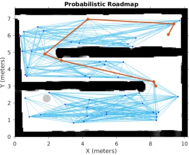
3.6. Instance of Probabilistic Roadmaps (PRM) with 50 nodes. . . 29
3.7. Geometry of the pure pursuit algorithm. . . 30
4.1. Flowchart of the proposed algorithm. . . 33
4.2. Introductory, simple maze developed in Gazebo simulator. . . 34
4.3. Right and centre bumper hit events. . . 35
4.4. Left and centre bumper hit events. . . 35
4.5. Bumper hit events by real Turtlebot. . . 35
4.6. Positions of obstacles in LASER scan area. . . 39
4.7. Fuzzy logic design. . . 40
4.8. Membership function plots for minimumRange. . . . 41
4.9. Membership function plots for CorrespondingAngle.. . . 42
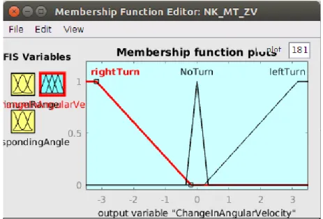
4.10. Membership function plots for ChangeInAngularVelocity.. . . 43
4.11. Rule base of the fuzzy controller. . . 43
4.12. The model of the system in MATLAB-Simulink. . . 44
4.13. MATLAB functionfcn. . . . 45
4.14. The Gazebo’s playground.world. . . . 46
4.15. Robot paths with and without obstacles. The blue path is observed in the presence of the obstacles and the red path is received in the absence of the obstacles. . . 47
4.16. Robot navigation model in Simulink. . . 50
4.17. Sugeno-type Fuzzy Inference System (FIS) obtained using ANFIS. . . 52
4.18. Training data and FIS output in neuro-fuzzy designer. . . 53
4.19. Membership function plots for input1 in Sugeno-type FIS. . . 54
4.20. Membership function plots for input2 in Sugeno-type FIS. . . 54
4.21. Sugeno-type fuzzy rules received using ANFIS. . . 55
4.22. Paths followed by the robot in simulated world. . . 56
4.23. Path followed by real robot in real world environment. . . 57
5.1. Simulated world in Gazebo. . . 62
5.2. Robot path generated from odometer measurements. . . 64
5.3. Standard deviation of scan ranges. . . 64
5.4. Robot navigation model in Simulink. . . 69
5.5. Simulated Turtlebot robot in a Gazebo world. . . 70
5.6. Repetitive paths followed by robot (using the proposed model given in Fig. 5.4) in Gazebo world. . . 71
5.7. Path followed by robot using advanced Algorithms 7−8. . . 74
5.8. Robot path based on the applied t-test. . . 80
A.1. Command to bring-up the corridor.world in ROS. . . 101
A.2. The corridor.world in Gazebo. . . 101
A.3. An instance of ROS topics list. . . 102
A.4. Turtlebot tele-operator command. . . 103
A.5. The Teki_test_nodein case of the Gazebo Simulator. . . 104
A.6. The Teki_test_nodein case of real robot. . . 104
A.7. Program to receive odometer information from robot. . . 109
A.8. Data file of way-points received from program given in Fig. A.7. . . 110
2.1. MATLAB releases and Toolboxes used. . . 9
3.1. Goal cell IDs and their coordinates used for Tables 3.2−3.4. . . 22
3.2. Planner time, path length and number of cells to visit using octile distance heuristic. . . 22
3.3. Planner time, path length and number of cells to visit using Euclidean distance heuristic. . . 23
3.4. Planner time, path length and number of cells to visit using Manhattan distance heuristic. . . 24
4.1. Description of the program instructions used in Fig. 4.13. . . 45
4.2. Coloured paths and Fuzzy Inference Systems (FISs) used in the Fig. 4.22. 56 5.1. Description of variables and initialized values . . . 63
5.2. LASER scan range vectors matches and robot positions . . . 66
5.3. Variables’ descriptions for Algorithms 6−8. . . 72
5.4. Initialization of variables for the Algorithms 6−8. . . 75
A.1. Description of the program instructions used in Fig. A.7.. . . 109
A.2. Critical values of tat 1% and 5% levels of significance. . . 112
1. Learning phase of PRM. . . 28
2. The path pursuit algorithm . . . 31
3. The x, y and z components of linear and angular velocities. . . 34
4. The robot navigation algorithm . . . 45
5. Obstacle recognition using LASER sensor and odometer . . . 61
6. Obstacles avoidance algorithm . . . 70
7. Obstacles recognition and avoidance algorithm . . . 73
8. Procedure to reverse the angular velocity of the robot . . . 74
9. Procedure to perform t-test on two independent range-vectorsx and y.. . 79
ANFIS Adaptive Neuro-Fuzzy Inference System ANN Artificial Neural Network
ANNs Artificial Neural Networks FIS Fuzzy Inference System FISs Fuzzy Inference Systems MF Membership Function
NDT Normal Distribution Transform PRM Probabilistic Roadmaps
ROS Robot Operating System
SLAM Simultaneous Localization and Mapping
1.1. Background of the research
Mobile robots have a wide range of applications like space missions, household and office work, receiving-delivering orders of clients in restaurants, transportation of logistics in inventories, inspection and maintenance, agriculture, security and defence, operations in radioactive areas etc. Mobile robots are very useful in the area where either the task is boring due to the repetitiveness of the same operations or the working environment is hazardous for the human being. For mobile robots, the navigation from one location to the other is one of the most desirable operations [1–4]. On the basis of the available prior information, the navigation environments can be classified into two major types:
known environment and unknown environment. Further, the navigation environments may or may not change during the navigation task. Generally, for the navigation point of view, the navigation environments get changes due to the moving obstacles. Therefore, a navigation environment is considered as static if the obstacles in the path are static. On contrast, a navigation environment is dynamic if the obstacles are dynamic. Consequently, the applicable navigation strategies depend on the type of the navigation environment [5–7].
The navigation process can be subdivided into two parts: global navigation and local navigation. The global navigation method is used to find globally optimal path on the basis of prior information like map of the environment. However, in the absence of sufficient prior information the global navigation strategy is not applicable. Instead of the prior information, the local navigation is based on the on-line sensory data received from the sensors mounted on the robot. Therefore, the local navigation methods can also be applied when the navigation environment is unknown or partially known. In real-world scenarios, support vector machinesbased local planner can be efficiently integrated into an autonomous navigation system [8]. Global path planner and local path planner are the two main parts of the navigation system of autonomous robot. These two path planners, in cooperation, make the robot motion optimal and collision free. The global planner generates a feasible route from the robot’s current location and orientation to the goal
location and orientation. The local path planner moves the robot as per the global plan and dynamically adapts to dynamic environment state [9–12].
In known environments, path planning is the process of finding the best feasible path from start to goal location [13–16]. In addition, self localization and mapping are among the challenging tasks [NK-17]. Simultaneous Localization and Mapping (SLAM)yields a map of the environment and keeps track of the robot in the navigation environment with various objects [18–20]. SLAMand path planning are necessary for the autonomous navigation process [21]. A path planning algorithm to calculate convenient motions of the robot by taking the different optimization criteria like time, energy and distance into account to overcome unknown and challenging obstacles is proposed in [22]. In known and static environment, the robot navigation process can have four major steps: making the map of surrounding world, store the map in computer readable form, find a feasible path from start to goal in the stored map and then drive the robot on the observed path.
The process of map building includes the following three steps:
(i) Select the appropriate two-dimensional coordinate points in the environment world covering the whole working area.
(ii) Drive the robot following these selected coordinates, and receive the sensor readings.
(iii) In the occupancy grid framework, mark the free and occupied spaces in the world by setting the probabilities of occupied spaces as one and the probabilities of free spaces as zero.
The occupancy grid can be saved and used directly in robot path planning in a convenient way [23]. Representation of navigation environment as a grid-based space is a necessary task for robust and accurate motion planning of robot. A two-dimensional occupancy grid can be constructed using the data of LASER sensor before the execution of the motion planning function [24]. Many researchers used the occupancy grid representation of the environment world map in the robot navigation related work as in [25–28]. The occupancy grid map is computer readable and this map can be supplied to the computer program to find an obstacle free path. Recently, these concepts are used in [29,30]. A minimum cost path can be acquired by applying a classical approach [31]. For a mobile robot, bacterial potential field method can be used to compute the feasible, optimal and safe paths in environments with static and dynamic obstacles [32]. For real-time path planning in a complex and dynamic environment, a biologically inspired two level method gives the plus of both global and local path finding procedures [33].
Graph-based search algorithms may take larger computation time to find the globally optimal path because these algorithms exhaustively explore the search space. In this
case, a heuristic function increases the speed of exploration process by providing the estimate of the cost of reaching the goal node [34]. Useful heuristic functions for A*
algorithm can be obtained using the various distances given in [35]. In a hierarchical path planning approach, the A* algorithm finds a geometric path speedily and various path points can be chosen as sub-goals for the second level. Theleast-squares policy iteration algorithm can be used to acquire a near-optimal local planning strategy to generate smooth trajectories in the second level. Consequently, an optimized path can be found by sequentially achieving the sub-goals generated in the first level [36,37]. The global map should only consider the obstacles which are persistent and larger than a definite area.
Inclusion of many small obstacles in the global map may lead to the larger complexity of the topological space. Homotopic A* algorithm, as path planner, is presented and compared with other path planners in [38]. However, the different heuristic functions are not taken into consideration in the implementation of A* algorithm as global path planner for the autonomous navigation of mobile robots.
Probabilistic roadmaps technique can be used to find a path from start to the goal point in occupancy grid map [39]. InPRM technique, the given number of nodes are created in the free space of occupancy grid and then these nodes are connected to each other within some threshold connection distance. Further, one path from the available connected paths from start to goal is selected. The process of sampling and node addition in PRMis given in [40]. Various path planning strategies can be found in recent research work [41, 42]. To drive the robot on the given path, a path following algorithm is required.
An implementation of pure pursuit path tracking algorithm with some limitations is presented in [43].
In unknown environments, the robot navigation becomes more challenging because no satisfactory information on the environment is available before starting the navigation process. Therefore, a global navigation path may not be generated. In this case, a local path from the current position to the goal position may provide a solution. Further, in the case of robot navigation in known environment, there may be situations where the obstacles are dynamic. So, the actual positions of the dynamic obstacles may not be measured accurately in global path planning. Furthermore, the partially known environment consists of known and unknown obstacles. In the case of unknown and dynamic environment, the robot needs to avoid the obstacles by using its inbuilt sensors.
A robot can not only avoid the obstacles but also find a globally optimal path by dynamically altering the locally optimal paths [44, 45]. In these cases, the local path planning is a suitable option for the navigation purpose [46]. In case of unknown environment, navigation task needs an approach that can work in uncertain situation [47].
The information about velocities of the dynamic obstacles is not necessarily required for the obstacle avoidance in the navigation path [48].
Modern control theory and robotics are advancing greatly due the development of new technologies [49]. Commonly, there are two steps in the design of the controllers for mobile robots. Firstly, the data from sensors are computed into high level and meaningful values of variables. Secondly, some machine learning method is used to produce a controller.
Taking these high level variables as input, the controller outputs the control commands for the robot [50].
Humans perform the navigation task without any exact computation and mathematical modelling. The ability of humans to deal with uncertainties can be followed in robot navigation using the neural network and fuzzy logic. Fuzzy logic gives an abstract behaviour of the system in an intuitive form even in the absence of precise mathematical and logical model. In practice, the sensor information is noisy and unreliable. The sensor inputs to the robot can be mapped into the control actions using fuzzy rules.
Therefore, fuzzy logic is a suitable tool to achieve robust robot behaviour [51]. The obstacles can be treated as integrated part of the environment. Human-like approaches to avoid the obstacles can be used in robot navigation [52]. In the environments with moving and deforming obstacles, a purely reactive algorithm to navigate a mobile robot mathematically guarantees collisions avoidance [53]. A fuzzy logic based navigation approach which uses grid based map and a behaviour based navigation method is given in [54]. However, this approach requires the environmental information in grid map in advance. In different conditions and uncertainty, an optimal and robust fuzzy controller for path tracking is presented in [55]. A Mamdani-type fuzzy controller [56] for wheeled robot can be optimal for trajectory tracking to deal with parametric and non-parametric uncertainties [57]. Neural networks have the ability to work with imprecise information and are excellent tools applicable in obstacle avoidance by mobile robots. Reliable and fault-tolerant control can be obtained with neural control systems [58]. In robot navigation, neural network can be employed to map the relationships between inputs and outputs for interpreting the sensory data, obstacle avoidance and path planning.
Although, the neural network method is slow and the learning algorithm used may not lead to an optimal solution. Thus, the integrated approaches like neuro-fuzzy technique are much more suitable for the robot navigation task [16]. In complex and unknown environments, simulation experiments indicate better navigation performance using neuro- fuzzy approach. Using neuro-fuzzy approach, the parameters of the controller can be optimized and the structure of the controller can be self-adaptive. To improve automatic learning and adaptation,ANFIS combines fuzzy logic and neural network. ANFIScan
be used to predict and model several engineering systems. ANFISis a fuzzy based model which is trained using some data set. Consequently, ANFIS computes the best suitable parameters of membership functions involved inFIS[59,60].
LASER scanner is one of the most common sensors used to execute SLAM [61–
63]. Using a LASER scan, the Normal Distribution Transform (NDT) can model the distribution of all two dimensional points around the robot. Two successive LASER scans can be aligned usingNDT to recover the translation and rotational parameters between the two scan positions. A map can be defined as the collection of LASER scans along with their global poses [64]. In the process of alignment of two LASER scans, the point of the LASER scan sample of the second scan in its coordinate frame is mapped into the first scan coordinate frame. Importantly, this mapping can be said optimal if the sum of the normal distributions of mapped points of second scan into first one using the mean and covariance of theNDTof the first scan is maximum. For autonomous robots [65,66], a survey on heuristic approaches in robot path planning is given in [16]. Artificial Neural Network (ANN) can compensate erroneous sensor data.
Moreover, theANNcan be trained during the SLAM[67]. Regardless of the uncertainties in the sensors observations, robot may navigate safely from start to goal [47]. Using range finder sensors (e.g. LASER scan sensors), the robot can navigate from start to goal with obstacle avoidance in unknown and dynamic environments environment [68].
The obstacle size and velocity vector of the unmanned surface vehicles can be used to achieve the obstacle avoidance. Moreover, fusion of more than one navigation algorithms can result more accurate outcomes [69]. The issue of obstacle avoidance is treated as an optimization problem in [70]. Previous experiences during the robot navigation are helpful to predict the path with obstacle avoidance of static and dynamic obstacles [71].
Various requirements of obstacle avoidance can be satisfied for the changing distance between robot and the obstacles [72–74].
The combination of several sensor systems is used in mobile robots. For making navigation decision, sensor fusion is the task of combining the information into a usable form [75]. The complex task of programming generally prevents the use of industrial robots to a large extent [76]. In addition, there may be situations in the autonomous navigation in an unknown environment [77] that certain sensors of the robot do not work properly or they are removed to minimize programming and system complexity.
The present study begins with the robot navigation task in known environment and then advances to the robot navigation in unknown environment.
1.1.1. Research gaps in the existing solutions
Considering the background of the research (Section 1.1), the research gaps for the dissertation can be given by the following points (i)−(iii):
(i) It is evident from the existing research work that the robot navigation task in case of known-static environment is less-complex than in the case of unknown-dynamic environment. Therefore, to begin with, classical path planning strategies such as A* algorithm and PRM can be studied in known-static environment. As yet, no significant comparison of application of various heuristic functions in A* algorithm has been done for path planning.
(ii) The existing research has established that the fuzzy logic based techniques are best suitable for uncertain data. So, in case of unknown-dynamic environment, fuzzy logic based robot navigation model becomes an exciting research point to be considered. Thus far, Robot navigation model using Mamdani-type FIS, Sugeno- types FIS, and ANFIS has not been presented to obtain obstacle avoidance in simulated as well as real world unknown-dynamic environment.
(iii) A search robot may need to navigate through all around the working area. Hence, to avoid the repetitive paths in unknown environment, a search robot should recognise the obstacles visited earlier. Till present, for obstacle recognition and avoidance,
“standard deviation” and the “t-test” have not been applied for a search robot in unknown environment.
1.2. Dissertation outline
The current chapter (Chapter 1) presents the basis and the state of the art of the study.
Chapter2presents the scientific methods applied in the research work. The Section2.1 gives the details of hardware and software used in the study. In Section2.2of the chapter, mathematical foundations, of applied soft-computing techniques, has been described.
Chapter 3 is about the robot navigation in known and static environment. In this chapter, two approaches have been implemented for robot navigation. Firstly, A*
algorithm has been applied and the results are compared for different heuristic functions.
Secondly, the robot navigation is performed using the probabilistic road-maps and finding an optimal path from start to goal.
Chapter4is concerned with the robot navigation in unknown and dynamic environment.
This chapter contains three Sections. In the Section4.1 , an algorithm using the bumper
events of the robot has been proposed for the obstacle avoidance. A model for robot navigation using Mamdani-typeFIS is presented in Section4.2. Section4.3is about the robot navigation with obstacle avoidance using fuzzy controller based on Sugeno-type FIS.
Chapter 5 is based on the robot navigation in unknown and static environments.
There are three sections in this chapter. In Section 5.1, obstacle recognition, during the robot navigation, is achieved by comparing the standard deviations of the LASER scans’ distance range vectors. By combining the standard deviations of the distance range vectors, robot positions and time of scans, an advanced algorithm, for obstacle avoidance and breaking of the repetitive paths loops, is presented in Section5.2. Section 5.3considers t-test to check out the similarity of two readings LASER scan. Consequently, the outcome of the t-test has been used for obstacle recognition and avoidance during the robot navigation.
Finally, in Chapter6, conclusion of the study, applicability of the obtained results, and future research scope based on the dissertation are provided.
The organisational structure of the dissertation is shown by Fig. 1.1.
Figure 1.1.: Structure of the dissertation.
methods applied in the research work
During the research work efficient combination of the already known algorithms and scientific methodologies such as A*, probabilistic roadmap search are applied to achieve the new research results.
2.1. Hardware and software used for experimental set-up
In case of hardware used, the experimental work is carried out on a general purpose laptop computer containing 4x Intel core i3- 2350M CPU @ 250-GHz and 3952 MB memory. A real Turtlebot robot is used to for testing the proposed methods. Turtlebot is a wheeled mobile robot. This robot kit is useful for the researcher due to its low cost and open source. The main hardware components of Turtlebot are Turtlebot Structure,Turtlebot Module Plate,Kinect, Robot Operating System (ROS) compatible Netbook, Asus Xion Pro Live, and Kobuki Base. In addition to the software development kit (SDK), the robotic software development environment of the Turtlebot provides libraries for the several useful tools like visualization, control and error handling. To bring up the Turtlebot in the real system, theROS command$ roslaunch turtlebot_bringup minimal.launch can be used in the Ubuntu (Operating System) terminal.
The main software used in the work are as follows:
• The operating system installed on the computer is Ubuntu, version 14.04.5 LTS.
The operating system has been updated toUbuntu 16.04.4 LTS in Section5.2.
• AsROS, Indigo distribution with version 1.11.20 is considered.
• To simulate the navigation task, Gazebo simulator version 2.2.6 is used till the Section5.1. Thereafter, the Gazebo version is updated to 7.0.
• For computer programming purpose,C++language is used in the Sections3.1and 4.1. In the remaining Sections, MATLAB is considered for the programming task.
Section-wise, MATLAB release version related Information is given in Table2.1.
Table 2.1.: MATLAB releases and Toolboxes used.
Section MATLAB release used Toolboxes used
3.2 R2016b Robotics System Toolbox
4.2 R2016b
Simulink,
Robotics System Toolbox, Fuzzy Logic Toolbox
4.3 R2016b Simulink,
Robotics System Toolbox
5.1 R2018a Robotics System Toolbox
5.2 R2018a Simulink,
Robotics System Toolbox
5.3 R2019a Robotics System Toolbox
2.2. Mathematical foundations of applied soft computing techniques
Modern soft computing tools, fuzzy logic, artificial neural networks, and neuro-fuzzy inference systems are also used in our work. The soft computing tools serve as approximate technical realization of the universal approximators (e.g. [78–80]).
2.2.1. Artificial neural network (ANN)
An artificial neuron (perceptron) mimics the computational function of biological neuron.
Fig.2.1 shows a model of artificial neuron presented by [81].
Figure 2.1.: Artificial neuron model given by [81].
The output (vj) of an artificial neuron can be defined using (2.1).
uj =
n
X
i=1
ωjiai+bj vj =φ uj
(2.1)
where,
bj = bias or offset for jth neuron in the layer.
ωji = synaptic weights for jth neuron in the layer.
ai = input to the neuron
Multilayer perceptron (a feedforward neural network) is layered network of artificial neurons. To obtain parallel computation, a layer of theANN consists several artificial neurons. In each layer of this type ofArtificial Neural Networks (ANNs), functions of the artificial neurons are similar. The output of the neurons in a layer is passed to the neurons of the next layer. This network type is applicable for the approximation of non-linear multiple variable functions by supervised training that means setting the number of neurons in the layers, and following that, setting the connection weights and biases by minimizing the mapping error for the samples used for training. Inerror backpropagation [82] learning, thegradient descent method is used for training the network. In our work, multilayer perceptron, witherror backpropagation learning, has been applied.
In other types of ANNs, recurrent neural networks (e.g. Hopfield’s and Elman’s networks [83, 84]) that can model system’s dynamics, convolutional neural networks that have come into fashion recently for recognizing typical patterns in various scales in strongly non-linear processes e.g. in fluid dynamics [85] and work on the basis of the approximation abilities of the Volterra Polynomials [86], or self-organizing mapsas Kohonen’s network (e.g. [87]) that can learn without supervision. However, these type of ANNs are not applied in our work.
2.2.2. Fuzzy logic 2.2.2.1. Fuzzy set
Ordinary sets have a limited scope of applicability. In real life problems, the ordinary set are not well suited to define the membership of objects in case of human thinking.
An ordinary set can also be defined usingMF. The membership function of an ordinary subsetY of the setU (universe of discourse) can be defined as follows:
χY :U → {0,1}
χY (x) =
0, x /∈Y 1, x∈Y
(2.2)
This definition of ordinary sets is extended for the fuzzy sets using the membership function. According to [88], in a fuzzy set, objects have continuum membership function values. Fuzzy setYe can be defined by (2.3), as follows:
Ye =
x, µ
Ye(x):x∈U
. (2.3)
where, x, µ
Ye(x) is ordered pair of an element (x) and the actual value of its corre- sponding membership functionµ
Ye(x). The membership function values range between zero and oneµ
Ye(x) :U →[0,1]. Support
suppYe
and core
coreYe
ofYe can be expressed by (2.4) as follows:
suppYe=nx∈U |µ
Ye(x)>0o, coreYe=nx∈U |µ
Ye(x) = 1o,
(2.4)
Various generalizations of the classical AND, and OR operators are developed for the fuzzy sets, on the basis of which the fuzzy inference systems can be elaborated. Also, various generalizations of the classical negation operator (¬) can be elaborated, and the statements of the De Morgan’s Laws can be maintained for fuzzy sets (e.g. [89–91]).
2.2.2.2. Membership functions
Inπ-shaped fuzzy sets, the membership function increases from zero to a maximum (≤1) and after reaching maximum it decreases to zero. This type of membership functions are used to present the fuzzy concepts like: ‘around’, ‘approximately’, ‘close to’.
The well known membership functions forπ-shaped fuzzy sets arebell, triangle, and trapezoid. A triangle membership function can be defined using (2.5).
µ(x) =
0, for (x≤p) or (x≥q)
x−p
a−p, forp≤x≤a
q−x
q−a, fora≤x≤q
(2.5)
where, the interval [p, q] and the pointaare support and core of the MF, respectively.
Fig. 2.2 shows a triangle MF by taking the values of parameters as indicated in its caption. If the membership occurs at a point then triangle membership function is widely used. When the membership occurs in domain then the trapezoid membership function is applicable. Fig.2.3 represents a trapezoidMFincluding the values of its parameters.
Figure 2.2.: TriangleMFhaving support and core as [2,7] and 5, respectively.
Figure 2.3.: Trapezoid MF by taking support and core intervals as [1,11] and [4,8], respectively.
The trapezoid membership function can be defined by (2.6).
µ(x) =
0, for (x≤p) or (x≥q)
x−p
a−p, forp≤x≤a 1, fora≤x≤b
q−x
q−b, forb≤x≤q
(2.6)
where, the intervals [p, q] and [a, b] are support and core of the MF, respectively.
As non-linear membership functions, bell MFand GaussianMF are widely used.
Figure 2.4.: Generalized bellMFby taking w= 6, s= 8,c= 10.
Figure 2.5.: Gaussian MFhaving values of the parameters asσ= 2, m= 10.
The generalised bell membership function is defined in (2.7) as follows:
µ(x) = 1 1 +x−cw 2s
(2.7)
where,
w defines the width of theMF.
sdefines the curve-shape on both sides of the plateau.
c= center of the MF.
Shape of a generalized bell MF, with the values of parameters as w= 6, s= 8, c= 10, is given in Fig. 2.4.
Gaussian membership function can be defined as given in (2.8).
µ(x) =e
−(x−m)2
2σ2 (2.8)
where, m and σ are the mean and the standard deviation, respectively.
2.2.3. Fuzzy inference system
A model of FISis presented in Fig. 2.6. In Fig.2.6, the input and theoutput are crisp values.
Figure 2.6.: A model of fuzzy inference system presented in [92].
Theinference unitof the fuzzy inference system takes decisions by using theIF. . . THEN rules provided by the knowledge base. There are the following two main methods ofFIS:
(i) Mamdani FIS[93].
(ii) Takagi-SugenoFIS(also known as SugenoFIS) [94].
2.2.3.1. Fuzzification
Fuzzification is a mapping of a point (real-valued)x∗ ∈U ⊂Rto a fuzzy set Ye ∈U. The widely used fuzzification methods are singleton fuzzifier, Gaussian fuzzifier, and triangular fuzzifier.
(i) Singleton fuzzifier:
µ
Ye(x) =
1, ifx=x∗ 0, otherwise
(2.9)
(ii) Gaussian fuzzifier:
µ
Ye(x) =e− x
1−x∗ 1 c1
2
? e− x
2−x∗ 2 c2
2
? . . . ? e− xn−x∗
n cn
2
(2.10) where, {ci, i= 1, . . . , n} are positive constants and the operator ?corresponds to some “generalized AND operator”. Usually,?is min or algebraic product.
(iii) Triangular fuzzifier:
µ
Ye(x) =
1−|x1−x∗1|
c1
? . . . ?
1−|xn−x∗n|
cn
, if xi−x∗i≥ci, fori= 1 to n.
0, otherwise
(2.11) where, ci and ?have the same meaning as in (2.10).
2.2.3.2. Defuzzification
LetYe is a fuzzy set defined overU with its membership functionµ
Ye(x), x∈U, and letx∗ denotes the defuzzification ofµ
Ye(x). Main methods to obtain x∗ arecentroid of gravity, center of sum method, mean of max method, height method,bisector defuzzification, smallest of maximum defuzzification, largest of maximum defuzzification, andweighted average defuzzification method.
The center of gravity method is given in (2.12).
x∗ = R xµ
Ye(x)dx Rµ
Ye(x)dx (2.12)
where, Rµ
Ye(x)dxis the area bounded byµ
Ye andx∗ represents x-coordinate of the center of gravity of the area.
If the membership function has n different disjoint peaks then the center of sum method, defined in (2.13), can be applied.
x∗ = Pn
i=1xiA
Yei
Pn i=1A
Yei
(2.13)
here,A
Yei represents area bounded by the Yei andxi denotes geometric center of the area.
Weighted average method is also known asSugeno defuzzification method. The crisp output using this method is presented in (2.14).
x∗ = Pn
i=1xiµ
Yei(xi) Pn
i=1µ
Yei(xi) (2.14)
where, xi is the middle value of theith peak, Yei(x).
2.2.4. Adaptive neuro-fuzzy inference system (ANFIS) Neuro-fuzzy systems combine:
(i) the learning and parallel computational abilities of neural networks,
(ii) human-like comprehension and knowledge representation of the fuzzy systems.
Adaptive network is a superset of feed-forward neural networks having supervised learning.
Fuzzy rules of ANFISare developed using Sugeno FIS [94]. Form of a Sugeno fuzzy rule for can be given as (2.15).
Rule: If xis Xi and/or y isXj then z=f(x, y) (2.15) The function f(x, y), in (2.15), is defined by (2.16) as follows:
f(x, y) =
d, for zero-order SugenoFIS ax+by+c, for first-order SugenoFIS
(2.16)
where, {a, b, c} is the set of parameters. x,y are input variables and Xi, Xj are fuzzy sets for i, j = 1 ton. n represents total number of fuzzy sets for the input and dis a constant.
Figure 2.7.: A four-rule-ANFIS Structure using the model of [92].
Layer structure of a four-rule-ANFIS(Fig.2.7) can be given by usingANFISmodel of [92].
The functions of nodes in thelayer 1 are similar as given in (2.17):
Oi(1)=µXi(x) (2.17)
where,
x= input to node i.
Xi= corresponding linguistic label of the node for i= 1 to n.
n= total number of nodes in thelayer 1.
µXi = membership function ofXi. According to need, the membership function µXi
can be selected from the definitions given in (2.5), (2.6), (2.7), (2.8).
In the layer 2, each node multiplies its input values. The output of a node inlayer 2 is defined as (2.18).
ui=µXj(x)×µXk(y) (2.18)
where, the operator× is generalised AND.
In case of ANFIS structure given in Fig.2.7,i= 1 to 4,j = 1,2, andk= 3,4.
Output of each node represents rule’s firing strength.
In the layer 3, the output ofithnode is ratio of firing strength ofith rule to the sum of the firing strengths of all rules, as given in (2.19).
vi = ui Pn
k=1uk
(2.19) where, n is the total number of rules in the ANFIS.
The output of ith node in the layer 4 is defined in (2.20).
O(4)i =vizi, fori= 1 ton. (2.20) where, nis the total number of rules in the ANFIS structure.
Thelayer 5 has single node. The output (z) of this layer can be expressed as in (2.21).
z=
n
X
i=1
vifi, fi =aix+biy+ci,
(2.21)
where, {ai, bi, ci}is the set of parameters for ith rule, and nis the total number of rules in theANFIS structure [92,94].
avoidance in known and static environment
3.1. Heuristic approaches in robot navigation
This section presents the implementation of A* algorithm as a global path planner for the navigation of a Turtlebot robot. A map of the navigation environment has been developed for a Gazebo simulator’s world. Manhattan distance, octile distance, and Euclidean distance heuristic functions are used to estimate the cost of moving from a cell to the goal cell of the environment. Time taken by the global planner, length of the path covered and the number of cells to visit are presented in tabular form. Mat plots for global costmap changes are also given using ‘rqt’ tool of ROS.
Considering the different heuristic functions, the A* algorithm has been implemented for the autonomous navigation of Turtlebot robot. For the local planner, the default dynamic window approach of ROSis used.
Remaining part of this section is organized as follows: Mathematical background of A* algorithm and the different heuristic functions used are given in Section 3.1.1.
Section3.1.2 presents the implementation and results of the study. Finally, Section3.1.3 is for the summary of the work.
3.1.1. A* algorithm and the heuristic functions
The A* algorithm provides the solution by searching among all possible paths and selects the path that minimizesf(x1, y1), the sum of the cost of the path from the start node to the node (x1, y1) and estimated cost of the cheapest path from the node (x1, y1) to the goal node [34].
f(x1, y1) =g(x1, y1) +h(x1, y1), (3.1) where, g(x1, y1) is the cost of the path from the start node to (x1, y1), andh(x1, y1) is a heuristic that estimates the cost of the cheapest path from (x1, y1) to the goal.
Let|x|represent the absolute value of x andC represent the minimum cost of moving from one space to adjacent space. Various distance metrics and distances including the following are given in [35].
The Manhattan distance heuristic function is expressed in (3.2) as follows:
h(x1, y1) =C(|x1−x2|+|y1−y2|), (3.2) The diagonal distance heuristic is defined in (3.3) as follows:
h(x1, y1) =C(|x1−x2|+|y1−y2|) + (D−2C) M in(|x1−x2|,|y1−y2|), (3.3) In (3.3),M in(|x1−x2|,|y1−y2|) gives the minimum value between the two arguments andD represents the cost of moving diagonally. The diagonal distance is calledoctile distance when C= 1 and D=√
2.
The Euclidean distance heuristic is given by (3.4).
h(x1, y1) =Cp(x1−x2)2+ (y1−y2)2, (3.4) 3.1.2. Implementation and experimental results
The A* algorithm is implemented in C++ for the three heuristic functions (3.2)−(3.4) given in Section3.1.1. Methods to create user-defined Gazebo-world and to make commu- nication between software packages usingROS are provided in AppendicesA.1and A.2, respectively. An introduction to pre-defined and user-defined ROSnodes is provided in AppendixA.3. ROSpackages based method to create map of the navigation environment and robot’s autonomous navigation with given map are explained in Appendix A.5.
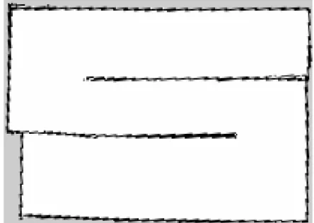
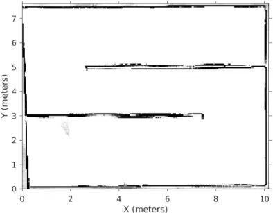
Usinggmapping package ofROS, map ofcorridor.world (Fig. A.2) is built. Description about the corridor.world is given in Appendix A.1.2. Fig. 3.1 represents the map of corridor.world.
Fig.3.2represents the global costmap updates for the map presented in Fig. 3.1. The costmapis a data structure which provides the information of the safe places for the robot navigation. Thecostmap uses sensor data from the world to produce an occupancy grid map. The globalcostmap is applicable in global navigation. In Fig. 3.2, the description of variables is as follows:
‘/move_base/global_costmap/costmap_updates/height’ = map height
‘/move_base/global_costmap/costmap_updates/width’ = map width
‘/move_base/global_costmap/costmap_updates/x’ = map’s x origin (in global frame)
‘/move_base/global_costmap/costmap_updates/y’ = map’s y origin (in global frame)
here, the measurement unit of the variables is meter.
Due to erroneous sensor data, the height and width of the map produced varies slightly during the map building process.
Figure 3.1.: Map of corridor.world using gmapping package of ROS.
Figure 3.2.: Global costmap updates forcorridor.world
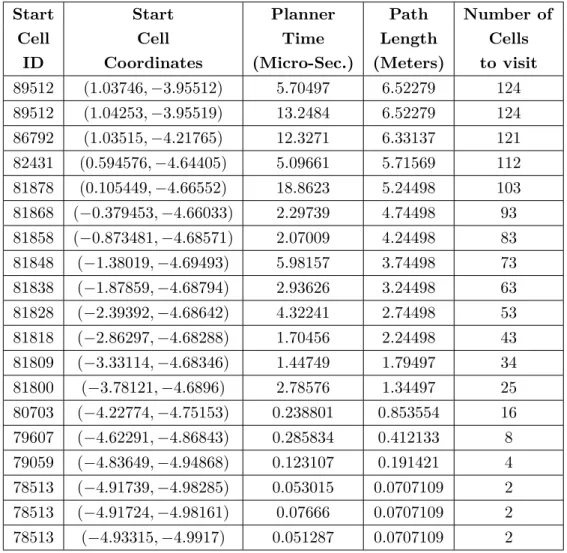
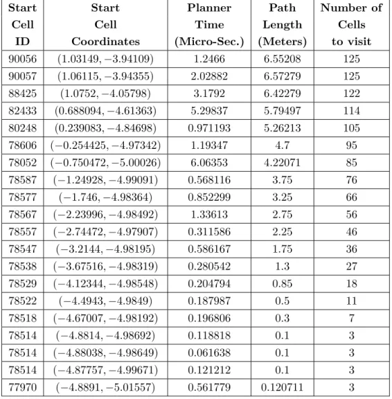
The costmap allocates an unique ID (Cell ID) to each cell of the occupancy grid map. The two-dimensional coordinates of the center of a cell are considered as the cell coordinates of that cell. Tables 3.2−3.4 provide the details of visited cell coordinates, current and goal cell IDs, global planner time to reach the goal cell from the current cell,
estimated distance from current cell to goal cell in meters and number of cells to visit using octile distance, Euclidean distance and Manhattan distance heuristics, respectively.
Goal cell IDs and corresponding goal coordinates used for Tables3.2−3.4 are given in Table3.1.
Table 3.1.: Goal cell IDs and their coordinates used for Tables 3.2−3.4.
Table Number Goal Cell ID Goal Cell Coordinates (X2, Y2)
3.2 78511 (−5.01013,−4.96942)
3.3 77968 (−4.99168,−5.00425)
3.4 78512 (−4.99091,−4.99587)
Table 3.2.: Planner time, path length and number of cells to visit using octile distance heuristic.
Start Start Planner Path Number of
Cell Cell Time Length Cells
ID Coordinates (Micro-Sec.) (Meters) to visit 89512 (1.04364,−3.95498) 0.973915 6.55208 125
89513 (1.0669,−3.95554) 2.04848 6.57279 125
87336 (1.03579,−4.17968) 1.68727 6.38137 122
81344 (0.610965,−4.70829) 1.15402 5.75355 114 79159 (0.164069,−4.90315) 0.961782 5.22071 105
78605 (−0.326765,−4.98568) 1.75893 4.7 95
78595 (−0.82855,−4.99297) 0.728234 4.2 85
78585 (−1.33259,−4.98773) 0.782637 3.7 75
78575 (−1.83213,−4.98842) 0.650034 3.2 65
78565 (−2.33186,−4.98401) 0.93469 2.7 55
78555 (−2.81918,−4.97933) 0.406216 2.2 45
78545 (−3.30742,−4.98043) 0.688205 1.7 35
78536 (−3.75951,−4.98735) 0.312633 1.25 26
78527 (−4.21368,−4.985) 0.110972 0.8 17
78520 (−4.5861,−4.98205) 0.166721 0.45 10
78516 (−4.7804,−4.98784) 0.062063 0.25 6
78513 (−4.93287,−4.99858) 0.11679 0.1 3
77969 (−4.93267,−5.00009) 0.056646 0.120711 3 77969 (−4.93653,−5.01733) 0.066747 0.120711 3
It is clear from the data of the Tables3.2−3.4that the planner time taken to move the robot from current cell to next cell using Manhattan distance heuristic changes moderately during the navigation. In the case of octile distance heuristic, the global planner time, taken for cell transitions during the robot navigation, changes swiftly. The global planner time for robot navigation from one cell to the next cell of the path is varying largely. Own publication related to Section3.1 is given in [NK-95].
Table 3.3.: Planner time, path length and number of cells to visit using Euclidean distance heuristic.
Start Start Planner Path Number of
Cell Cell Time Length Cells
ID Coordinates (Micro-Sec.) (Meters) to visit
89512 (1.03746,−3.95512) 5.70497 6.52279 124
89512 (1.04253,−3.95519) 13.2484 6.52279 124
86792 (1.03515,−4.21765) 12.3271 6.33137 121
82431 (0.594576,−4.64405) 5.09661 5.71569 112 81878 (0.105449,−4.66552) 18.8623 5.24498 103 81868 (−0.379453,−4.66033) 2.29739 4.74498 93 81858 (−0.873481,−4.68571) 2.07009 4.24498 83 81848 (−1.38019,−4.69493) 5.98157 3.74498 73 81838 (−1.87859,−4.68794) 2.93626 3.24498 63 81828 (−2.39392,−4.68642) 4.32241 2.74498 53 81818 (−2.86297,−4.68288) 1.70456 2.24498 43 81809 (−3.33114,−4.68346) 1.44749 1.79497 34
81800 (−3.78121,−4.6896) 2.78576 1.34497 25
80703 (−4.22774,−4.75153) 0.238801 0.853554 16 79607 (−4.62291,−4.86843) 0.285834 0.412133 8 79059 (−4.83649,−4.94868) 0.123107 0.191421 4 78513 (−4.91739,−4.98285) 0.053015 0.0707109 2 78513 (−4.91724,−4.98161) 0.07666 0.0707109 2 78513 (−4.93315,−4.9917) 0.051287 0.0707109 2
Table 3.4.: Planner time, path length and number of cells to visit using Manhattan distance heuristic.
Start Start Planner Path Number of
Cell Cell Time Length Cells
ID Coordinates (Micro-Sec.) (Meters) to visit
90056 (1.03149,−3.94109) 1.2466 6.55208 125
90057 (1.06115,−3.94355) 2.02882 6.57279 125
88425 (1.0752,−4.05798) 3.1792 6.42279 122
82433 (0.688094,−4.61363) 5.29837 5.79497 114 80248 (0.239083,−4.84698) 0.971193 5.26213 105
78606 (−0.254425,−4.97342) 1.19347 4.7 95
78052 (−0.750472,−5.00026) 6.06353 4.22071 85
78587 (−1.24928,−4.99091) 0.568116 3.75 76
78577 (−1.746,−4.98364) 0.852299 3.25 66
78567 (−2.23996,−4.98492) 1.33613 2.75 56
78557 (−2.74472,−4.97907) 0.311586 2.25 46
78547 (−3.2144,−4.98195) 0.586167 1.75 36
78538 (−3.67516,−4.98319) 0.280542 1.3 27
78529 (−4.12344,−4.98548) 0.204794 0.85 18
78522 (−4.4943,−4.9849) 0.187987 0.5 11
78518 (−4.67007,−4.98192) 0.196806 0.3 7
78514 (−4.8814,−4.98692) 0.118818 0.1 3
78514 (−4.88038,−4.98649) 0.061638 0.1 3
78514 (−4.87757,−4.99671) 0.121212 0.1 3
77970 (−4.8891,−5.01557) 0.561779 0.120711 3 3.1.3. Summary
The three different heuristic functions are used in the implementation of A* algorithm as a global path planner for the Turtlebot robot. It is observed that the coordinates of the cells on the path generated by each of the heuristic function do not differ significantly.
Nevertheless, the time taken by global path planner, with different heuristic function used, differ significantly. Among the three, the Euclidean distance heuristic produces the most non-uniform global path planner time for the transition of the robot between the cells during navigation. On the other hand, octile distance heuristic depicts the most uniform behaviour for the global path planner time throughout the navigation path.
![Figure 2.2.: Triangle MF having support and core as [2, 7] and 5, respectively.](https://thumb-eu.123doks.com/thumbv2/9dokorg/515035.195/34.892.269.617.625.898/figure-triangle-mf-having-support-core-respectively.webp)