Theses Booklet (Main ﬁndings in the Ph.D. dissertation)

(1)

Theses Booklet

(Main findings in the Ph.D. dissertation)

entitled:

“Robot Navigation in Unknown and Dynamic Environment”

by:

Neerendra Kumar

(Ph.D. Student)

Supervisor:

Dr. Zoltán Vámossy

(Associate Professor)

Doctoral School of Applied Informatics and Applied Mathematics

Budapest, 2020

(2)

research work. He always responded my queries, emails and paper corrections very quickly. Further, my supervisor, always supported me, promptly, about the document requirements of the Universities pertaining to this study. I have always got positive response from him for our meetings to discuss the research problems and the possible solutions.

I am greatly thankful toProf. Aurél Galántai, the head of theDoctoral School of Applied Informatics and Applied Mathematics of theÓbuda University, for his immense support and leadership to improve the results and to achieve the final goal of the work. I am highly thankful toProf. László Horváthfor his valuable and motivational comments on my oral presentations of end semester research reports and on my research paper presentations in various internal conferences. I am grateful toProf. Levente Kovácsfor his interesting and easy to grasp subject lectures and his continuous inspiration to attend the International conferences related to my work. From bottom of my heart, I am thankful to Prof. József K. Tarfor his knowledgeable subject lectures and his provocation to use open source software.

I wholeheartedly thankful toMr. Zsolt Miklós Szabó-Resch for providing me his technical expertise and guidance onLinux, robot operating system, Gazebo simulator and robot handling. My profound thanks to Dr. György Eignerfor sharing the important informations related Ph.D. degree procedure and formats of required documents and research reports. My sincere thanks toMs. Bácskai ZsuzsannaandMs. Hersics Katalinfor their administrative support throughout my study atÓbuda University.

I am greatly thankful to the governments of HungaryandIndiafor selecting me for theTempus Public Foundation’s prestigiousStipendium Hungaricum Scholarship Programmeto get admission in this Ph.D. programme.

A lot of thanks toProf. Ashok Aima, Vice Chancellor of Central University of Jammu, India, for granting me the study leave to pursue this Ph.D. study. I am grateful toProf. Lokesh Verma,Prof. Devanandand my fellow colleagues of Central University of Jammu for their support in the study leave.

I would also like to thank to all of those who are not namely listed here, like, my professors, many of my friends and colleagues from whom I got inspired and learnt a lot.

Finally, I give my heartily thanks to my loving family members for their support.

(4)

1 Background of the Research

Mobile robots have a wide range of applications like space missions, household and office work, receiving-delivering orders of clients in restaurants, transportation of logistics in inventories, inspection and maintenance, agriculture, security and defence, operations in radioactive areas etc. Mobile robots are very useful in the area where either the task is boring due to the repetitiveness of the same operations or the working environment is hazardous for the human being. For mobile robots, the navigation from one location to the other is one of the most desirable operations [1–4]. On the basis of the available prior information, the navigation environments can be classified into two major types:

known environment and unknown environment. Further, the navigation environments may or may not change during the navigation task. Generally, for the navigation point of view, the navigation environments get changes due to the moving obstacles. Therefore, a navigation environment is considered as static if the obstacles in the path are static. On contrast, a navigation environment is dynamic if the obstacles are dynamic. Consequently, the applicable navigation strategies depend on the type of the navigation environment [5–7].

The navigation process can be subdivided into two parts: global navigation and local navigation. The global navigation method is used to find globally optimal path on the basis of prior information like map of the environment. However, in the absence of sufficient prior information the global navigation strategy is not applicable. Instead of the prior information, the local navigation is based on the on-line sensory data received from the sensors mounted on the robot. Therefore, the local navigation methods can also be applied when the navigation environment is unknown or partially known. Global path planner and local path planner are the two main parts of the navigation system of autonomous robot. These two path planners, in cooperation, make the robot motion optimal and collision free. The global planner generates a feasible route from the robot’s current location and orientation to the goal location and orientation. The local path planner moves the robot as per the global plan and dynamically adapts to dynamic environment state [8–11].

In known environments, path planning is the process of finding the best feasible path from start to goal location [12–15]. In addition, self localization and mapping are among the challenging tasks [NK-16]. Simultaneous Localization and Mapping (SLAM) yields a map of the environment and keeps track of the robot in the navigation environment with various objects [17–19]. SLAM and path planning are necessary for the autonomous navigation process [20]. A path planning algorithm to calculate convenient motions of

(5)

the robot by taking the different optimization criteria like time, energy and distance into account to overcome unknown and challenging obstacles is proposed in [21]. In known and static environment, the robot navigation process can have four major steps: making the map of surrounding world, store the map in computer readable form, find a feasible path from start to goal in the stored map, and then drive the robot on the observed path.

The process of map building includes the following three steps:

(i) Select the appropriate two-dimensional coordinate points in the environment world covering the whole working area.

(ii) Drive the robot following these selected coordinates, and receive the sensor readings.

(iii) Mark the free and occupied spaces in the world by setting the probabilities of occupied spaces as one and the probabilities of free spaces as zero in the occupancy grid framework.

The occupancy grid can be saved and used directly in robot path planning in a convenient way [22]. Representation of navigation environment as a grid-based space is a necessary task for robust and accurate motion planning of robot. A two-dimensional occupancy grid can be constructed using the data of LASER sensor before the execution of the motion planning function [23]. Many researchers used the occupancy grid representation of the environment world map in the robot navigation related work as in [24–27]. The occupancy grid map is computer readable and this map can be supplied to the computer program to find an obstacle free path. Recently, these concepts are used in [28,29]. A minimum cost path can be acquired by applying a classical approach [30].

Graph-based search algorithms may take larger computation time to find the globally optimal path because these algorithms exhaustively explore the search space. In this case, a heuristic function increases the speed of exploration process by providing the estimate of the cost of reaching the goal node [31]. Useful heuristic functions for A*

algorithm can be obtained using the various distances given in [32]. In a hierarchical path planning approach, the A* algorithm finds a geometric path speedily and various path points can be chosen as sub-goals for the second level. The global map should only consider the obstacles which are persistent and larger than a definite area. Inclusion of many small obstacles in the global map may lead to the larger complexity of the topological space. Homotopic A* algorithm, as path planner, is presented and compared with other path planners in [33]. However, the different heuristic functions are not taken into consideration in the implementation of A* algorithm as global path planner for the autonomous navigation of mobile robots.

(6)

Probabilistic roadmaps technique can be used to find a path from start to the goal point in occupancy grid map [34]. In PRM technique, the given number of nodes are created in the free space of occupancy grid and then these nodes are connected to each other within some threshold connection distance. Further, one path from the available connected paths from start to goal is selected. The process of sampling and node addition in probabilistic roadmaps is given in [35]. A collision free path can be obtained through the path planning using PRM and can be applied to related research as used in [36–39].

Various path planning strategies can be found in recent research work [40,41]. To drive the robot on the given path, a path following algorithm is required. An implementation of pure pursuit path tracking algorithm with some limitations is presented in [42].

In unknown environments, the robot navigation becomes more challenging because no satisfactory information on the environment is available before starting the navigation process. Therefore, a global navigation path may not be generated. In this case, a local path from the current position to the goal position may provide a solution. Further, in the case of robot navigation in known environment, there may be situations where the obstacles are dynamic. So, the actual positions of the dynamic obstacles may not be measured accurately in global path planning. Furthermore, the partially known environment consists of known and unknown obstacles. In the case of unknown and dynamic environment, the robot needs to avoid the obstacles by using its inbuilt sensors.

A robot can not only avoid the obstacles but also find a globally optimal path by dynamically altering the locally optimal paths [43, 44]. In these cases, the local path planning is a suitable option for the navigation purpose [45]. In case of unknown environment, navigation task needs an approach that can work in uncertain situation [46].

The information about velocities of the dynamic obstacles is not necessarily required for the obstacle avoidance in the navigation path [47].

Modern control theory and robotics are advancing greatly due the development of new technologies [48]. Commonly, there are two steps in the design of the controllers for mobile robots. Firstly, the data from sensors are computed into high level and meaningful values of variables. Secondly, some machine learning method is used to produce a controller.

Taking these high level variables as input, the controller outputs the control commands for the robot [49].

Humans perform the navigation task without any exact computation and mathematical modelling. The ability of humans to deal with uncertainties can be followed in robot navigation using the neural network and fuzzy logic. Fuzzy logic gives an abstract behaviour of the system in an intuitive form even in the absence of precise mathematical and logical model. In practice, the sensor information is noisy and unreliable. The

(7)

sensor inputs to the robot can be mapped into the control actions using fuzzy rules.

Therefore, fuzzy logic is a suitable tool to achieve robust robot behaviour [50]. The obstacles can be treated as integrated part of the environment. Human-like approaches to avoid the obstacles can be used in robot navigation [51]. In the environments with moving and deforming obstacles, a purely reactive algorithm to navigate a mobile robot mathematically guarantees collisions avoidance [52]. A fuzzy logic based navigation approach which uses grid based map and a behaviour based navigation method is given in [53]. However, this approach requires the environmental information in grid map in advance. In different conditions and uncertainty, an optimal and robust fuzzy controller for path tracking is presented in [54]. A Mamdani-type fuzzy controller [55] for wheeled robot can be optimal for trajectory tracking to deal with parametric and non-parametric uncertainties [56].

Neural networks have the ability to work with imprecise information and are excellent tools applicable in obstacle avoidance by mobile robots. Reliable and fault-tolerant control can be obtained with neural control systems [57]. In robot navigation, neural network can be employed to map the relationships between inputs and outputs for interpreting the sensory data, obstacle avoidance and path planning. Although, the neural network method is slow and the learning algorithm used may not lead to an optimal solution. Thus, the integrated approaches like neuro-fuzzy technique are much more suitable for the robot navigation task [15]. In complex and unknown environments, simulation experiments indicate better navigation performance using neuro-fuzzy approach. Using neuro-fuzzy approach, the parameters of the controller can be optimized and the structure of the controller can be self-adaptive. To improve automatic learning and adaptation, Adaptive Neuro-Fuzzy Inference System (ANFIS) combines fuzzy logic and neural network. ANFIS can be used to predict and model several engineering systems. ANFIS is a fuzzy based model which is trained using some data set. Consequently, ANFIS computes the best suitable parameters of membership functions involved in Fuzzy Inference System (FIS) [58,59].

LASER scanner is one of the most common sensors used to execute SLAM [60–62].

Artificial Neural network (ANN) can compensate erroneous sensor data. Moreover, the ANN can be trained during the SLAM [63]. Regardless of the uncertainties in the sensors observations, robot may navigate safely from start to goal [46]. Using range finder sensors (e.g. LASER scan sensors), the robot can navigate from start to goal with obstacle avoidance in unknown and dynamic environments environment [64]. The obstacle size and velocity vector of the unmanned surface vehicles can be used to achieve the obstacle avoidance. Moreover, fusion of more than one navigation algorithms can

(8)

result more accurate outcomes [65]. The issue of obstacle avoidance is treated as an optimization problem in [66]. Previous experiences during the robot navigation are helpful to predict the path with obstacle avoidance of static and dynamic obstacles [67].

Various requirements of obstacle avoidance can be satisfied for the changing distance between robot and the obstacles [68–70].

The combination of several sensor systems is used in mobile robots. For making navigation decision, sensor fusion is the task of combining the information into a usable form [71]. The complex task of programming generally prevents the use of industrial robots to a large extent [72]. In addition, there may be situations in the autonomous navigation in an unknown environment [73] that certain sensors of the robot do not work properly or they are removed to minimize programming and system complexity.

2 Directions and Goals of the Research

Forn number obstacles, the environment can be classified in the following categories:

(i) Known and static environment:

Locations of the obstacles are prior known and the velocity ofi^th obstacle can be given as follows:

|v_i|= 0 fori= 1 to n,

n is known and will not change during the navigation task.

(ii) Known and dynamic environment:

Locations of the obstacles are prior known and the velocity ofi^th obstacle can be given as follows:

|v˙_i|= 0 fori= 1 to n,

nis known and any change in n is prior specified.

(iii) Unknown and static environment:

Locations of the obstacles are not prior known and the velocity of i^th obstacle can be given as follows:

|v_i|= 0 fori= 1 to n,

n is unknown but does not change during navigation.

(iv) Unknown and dynamic environment:

Locations of the obstacles are not prior known and the velocity of i^th obstacle can be given as follows:

(9)

|v_i| ≥0 for i= 1 to n,

nis unknown and may vary during the navigation. Moreover, the velocities are unknown.

• The robot navigation in unknown environments is more challenging in comparison to the static environments.

• Present study begins with the navigation in known and static environment, and then, advances to the navigation task in unknown environments.

2.1 Research gaps in the existing solutions

Considering the background of the research (Section 1), the research gaps for the dissertation can be given by the following points (i)−(iii):

(i) It is evident from the existing research work that the robot navigation task in case of known-static environment is less-complex than in the case of unknown-dynamic environment. Therefore, to begin with, classical path planning strategies such as A* algorithm and PRM can be studied in known-static environment. As yet, no significant comparison of application of various heuristic functions in A* algorithm has been done for path planning.

(ii) The existing research has established that the fuzzy logic based techniques are best suitable for uncertain data. So, in case of unknown-dynamic environment, fuzzy logic based robot navigation model becomes an exciting research point to be considered. Thus far, Robot navigation model using Mamdani-type FIS, Sugeno- types FIS, and ANFIS has not been presented to obtain obstacle avoidance in simulated as well as real world unknown-dynamic environment.

(iii) A search robot may need to navigate through all around the working area. Hence, to avoid the repetitive paths in unknown environment, a search robot should recognise the obstacles visited earlier. Till present, for obstacle recognition and avoidance,

“standard deviation” and the “t-test” have not been applied for a search robot in unknown environment.

(10)

3 Materials and Methods of Investigation

3.1 Robot navigation with obstacle avoidance in known and static environment

3.1.1 A* algorithm and the heuristic functions

The A* algorithm [31] provides the solution by searching among all possible paths. In A*, the cost f(x1, y1)of reaching the goal, via a node (x1, y1), is defined in (1).

f(x₁, y₁) =g(x₁, y₁) +h(x₁, y₁), (1) where, g(x1, y1) is the cost of the path from the start node to (x1, y1), andh(x1, y1) is a heuristic that estimates the cost of the cheapest path from (x₁, y₁) to the goal.

Let|x|represents the absolute value ofx andC represents the minimum cost of moving from one space to adjacent space. Various distance metrics and distances including the following are given in [32].

The Manhattan distance heuristic function can be given as follows:

h(x1, y1) =C(|x₁−x2|+|y₁−y2|), (2) The diagonal distance heuristic can be given as follows:

h(x1, y1) =C(|x₁−x2|+|y₁−y2|) + (D−2C) M in(|x₁−x2|,|y₁−y2|), (3) In (3), M in(|x₁−x₂|,|y₁−y₂|) gives the minimum value between the two arguments andD represents the cost of moving diagonally. The diagonal distance is calledoctile distance when C= 1 and D=√

2.

The Euclidean distance heuristic is given as follows:

h(x₁, y₁) =C^p(x₁−x₂)²+ (y₁−y₂)², (4) The above three different heuristic functions defined through (2)−(4) are used in the implementation of A* algorithm as a global path planner for the Turtlebot robot.

It is observed that the coordinates of the cells on the path generated by each of the heuristic function do not differ significantly. Nevertheless, the time taken by global path planner, with different heuristic function used, differ significantly. Among the three, the Euclidean distance heuristic produces the most non-uniform global path planner time for the transition of the robot between the cells during navigation. On the other hand,

(11)

octile distance heuristic depicts the most uniform behaviour for the global path planner time throughout the navigation path [NK-74].

3.1.2 Probabilistic roadmaps (PRM)

The PRM path planning method has two phases, namely,learning phaseandquery phase.

In the learning phase, for a given scene, a roadmap (a data structure) is generated in probabilistic manner. The generated probabilistic roadmap is saved as an undirected graph. The nodes of the graph represent collision-free configurations of the robot and the edges of the graph represent feasible paths. Local planner of the navigation system computes these paths. The learning phase of the PRM is summarized using Algorithm 1.

Initially, the graph G={N_G, E_G} is empty.

Algorithm 1 Learning phase of PRM.

1: N_G, E_G← {}

2: whiletrue do

3: r ← a randomly selected free configuration

4: N_r ← {r⁰ ∈N_G|D(r, r⁰)≤d_m}

5: N_G ←N_G∪ {r}

6: for allx←Nr, in ascending order ofD(r, x) do

7: if P(r, x) & ¬C(r, x) then

8: E_G ←E_G∪(r, x)

9: Update connected components of G.

10: end if

11: end for

12: end while

where,

d_m= Maximum threshold distance between r and r⁰.

P(r, x) returns whether a path, between r and x, is found by local planner.

C(r, x) returns whetherr andx belongs to the same connected component.

D(r, x) is defined in (5).

D(r, x) = max

p∈robotkp(x)−p(r)k, (5)

In (5),

p represents a point on in the robot.

p(r) = workspace position ofp when the robot is atr.

kp(x)−p(r)k= Euclidean distance between p(r) andp(x).

During the query phase, a query is generated to find a path between two collision free

(12)

configurations. Initially, the method generates a path from start and goal to other two nodes in the roadmap. Consequently, the graph is searched to find the connecting edges to these two nodes. Eventually, a feasible path from start to goal is received by concatenating the path segments. It is experienced that this method provides good results when larger time span is given in learning phase. Various components of the method can be tailored to increase the efficiency of this method [34]. The method is applicable to the static environments where the obstacles do not get change.

A PRM of the map of a simulated world using Turtlebot-Gazebo simulator is tuned up for the number of nodes taken in PRM and the connection distance between the nodes in it. The navigation algorithm is applied in robot navigation task.

Investigations on the implemented algorithm resulted in the observation that the chosen environment was found to be well treatable by the A* algorithm, but it was found to be

“difficult” for the “probabilistic roadmap” approach because a large number of randomly selected nodes was necessary for finding a path between the initial and the final points of the task [NK-75].

3.2 Robot navigation with obstacle avoidance in unknown and dynamic environment

3.2.1 Robot obstacle avoidance using bumper event

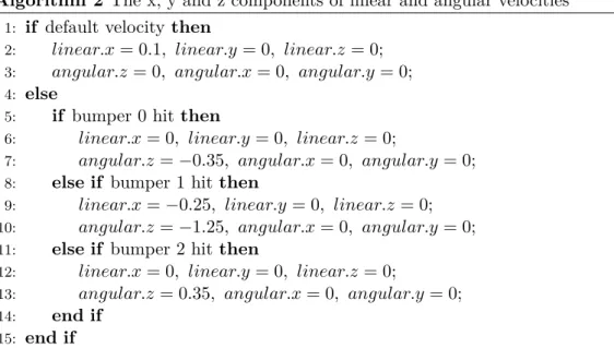
The implementation of the proposed Algorithm 2shows that the obstacle avoidance task can be handled by using the bumper events of the Turtlebot. The Turtlebot successfully recovers from the collisions and follows the new velocity commands. In the case of autonomous navigation in unknown environment, this algorithm is very useful when other sensors for obstacle avoidance are got damaged or removed to minimize the complexity.

The main disadvantage of the proposed algorithm is that it does not lead to a collision-free navigation. Therefore, the other sensors of robot like LASER and camera may get priority over bump sensor for collision-free navigation [NK-76].

(13)

Algorithm 2 The x, y and z components of linear and angular velocities

1: if default velocity then

2: linear.x= 0.1, linear.y= 0, linear.z= 0;

3: angular.z = 0, angular.x= 0, angular.y= 0;

4: else

5: if bumper 0 hitthen

6: linear.x= 0, linear.y= 0, linear.z= 0;

7: angular.z=−0.35, angular.x= 0, angular.y= 0;

8: else if bumper 1 hit then

9: linear.x=−0.25, linear.y = 0, linear.z= 0;

10: angular.z=−1.25, angular.x= 0, angular.y= 0;

11: else if bumper 2 hit then

12: linear.x= 0, linear.y= 0, linear.z= 0;

13: angular.z= 0.35, angular.x= 0, angular.y = 0;

14: end if

15: end if

3.2.2 Robot navigation in unknown and restricted dynamic environment using fuzzy control solutions

The pure pursuit algorithm [42] calculates the required curvature that can lead the robot from its current position to the goal position. The geometry of the pure pursuit algorithm is given in Fig. 1.

Figure 1: Geometry of the pure pursuit algorithm.

(14)

Pythagorean equation for the larger right triangle in Fig. 1, can be written as (6):

p²=x²+y². (6)

The line segments at the X axis of Fig. 1 hold the relation given in (7).

q=r−x. (7)

For the smaller right triangle of Fig. 1, Pythagorean equation can be presented by (8).

r² =q²+y². (8)

By solving (6) to (8), the curvature (ρ) of the path arc can be given by (9) as follows:

ρ= 1 r = 2x

p². (9)

The curvature of the path arc, obtained in (9), determines the steering wheel angle of the robot.

The robot navigation model is presented using MATLAB-Simulink software. Using publisher-subscriber strategy, the proposed model and the robot communicate with each other by passing specified messages on the relevant ROS topics. A publisher of the message sends the message on ROS topic. On the other side, the subscriber receives the message on the same topic from the ROS. In this model, the navigation task is accomplished by the following two controllers:

(i) The pure pursuit controller,

(ii) The fuzzy based controller (as described in Section3.2.2).

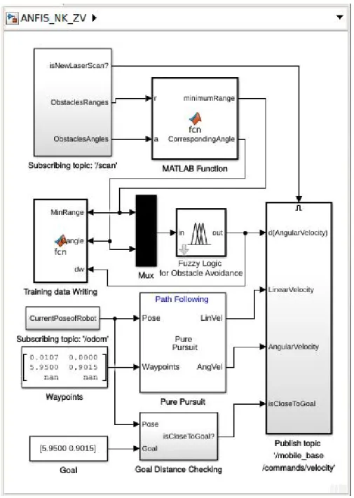
Fig.2 describes the details of the presented robot navigation model. This model contains four subsystems as follows:

(i) Subscribing topic: ‘/odom’, (ii) Subscribing topic: ‘/scan’, (iii) Goal Distance Checking,

(iv) Publishing topic: ‘mobile_base/commands/velocity’.

The robot publishes its position and orientation, in the environment, on the /odom topic of the ROS. The Subscribing topic: ‘/odom’ subsystem, in the given model, subscribes

(15)

the /odom topic of the ROS to obtain current pose of the robot. The robot publishes its LASER sensor scan readings vector on/scan topic in ROS.

Figure 2: Robot navigation model in Simulink.

A typical message vector on /scan topic contains distance ranges of obstacles in the scan area. In two dimensional state, the scan area is of ‘V’ shape. From right to left, a single LASER scan may contain some hundred ranges. Using minimum angle of scan and

(16)

angle increment, the corresponding angle to each range in a message can be find out. The obstacle ranges and their corresponding angles of scan, together, give the locations of the obstacles in the robot path. The Subscribing topic: ‘/scan’ subsystem is subscribing the ROS topic /scan to get the vectors of ranges and their corresponding scan angle.

Before sending the new velocity commands to the robot, theGoal Distance Checking subsystem checks the distance of goal from the current position of the robot. If the distance between the goal and the robot is less than or equal to the given value (in our case, it is 0.1 meter) then the new velocity commands will not be given to robot. As a result, the robot navigation process gets completed and, therefore, terminated.

The goal distance (p) between the goal position (x, y) and current position (x⁰, y⁰) of the robot can be expressed by (10) as given below:

p=^q(x−x⁰)²+ (y−y⁰)². (10) The linear and angular velocities commands are given to the robot by publishing geome- try_msgs/Twistmessage on the topic/mobile_base/commands/velocity of ROS. Robot is subscribing the topic /mobile_base/commands/velocity of ROS which is being published by the subsystem Publishing topic: ‘/mobile_base/commands/velocity’.

In addition to these subsystems, the remaining blocks of the model are as follows:

(i) two constant blocks named as Waypoints and Goal, (ii) aMux block,

(iii) aPure Pursuit path following algorithm block, (iv) two MATLAB functions,

(v) afuzzy logic for obstacle avoidance block.

TheWaypoints constant block is to contain a ‘N×2’ matrix of way points of navigation path . In case of unknown environment, it is considered that only start and goal positions of the robot are known, initially. The Goal constant block contains a two dimensional coordinates of goal position. TheMux block is combining the two inputs (minimumRange andCorrespondingAngle received from theMATLAB Function block) in a single output link. So that, these two input values can be passed to the fuzzy controller block by a single link. ThePure Pursuit block is used to compute the required linear and angular velocities to drive the robot using inputs from way-points of the path and current pose of the robot. Since the navigation environment is considered as unknown, the way-points of the feasible path are unknown except the two points: start and goal. The function

(17)

fcn in MATLAB Function block computes the minimum range and its corresponding angle of scan from the vectors of ObstaclesRanges and ObstaclesAngles received from Subscribing topic: ‘/scan’ subsystem block. The MATLAB function in theTraining data writing block is used to write the data in three separate columns for minimum range, its corresponding angle and the output from the fuzzy controller. This training data can be used to train a fuzzy inference system (FIS) using ANFIS model. The block named Fuzzy Logic for Obstacle Avoidance is a fuzzy logic controller block.

The published linear velocity is same as linear velocity given by the pure pursuit block. Since the pure pursuit block does not consider the obstacles in the path, the angular velocity is needed to be adjusted before its publication on the ROS. This required adjustment in the angular velocity is obtained by theFuzzy Logic for Obstacle Avoidance block. The published angular velocity (ω) can be stated by (11) as below:

ω=ω1+ω2. (11)

where,ω₁ is the angular velocity (i.e. AngVel) provided by path pursuit controller. ω₂ is the output (i.e. d(AngularVelocity)) of the fuzzy logic controller.

The fuzzy inference system (FIS) of the used fuzzy logic controller is considered as of the following two types:

(i) Mamdani-type FIS

(ii) ANFIS based Sugeno-type FIS

The membership functionsµ(x) taken in Mamdani-type FIS are defined using (12) and (13).

µ(x) =











0, forx≤p

x−p

a−p, forp < x≤a 1, fora < x≤b

q−x

q−b, forb < x≤q 0 forq < x

(12)

where, the parameters p andq are the feet of the MF and aandb are the shoulders of

(18)

the MF.

µ(x) =











0, forx≤p

x−p

a−p, forp < x≤a

q−x

q−a, fora < x≤q 0 forq < x

(13)

where, the parameters p and q are the feet of the MF and ais the peak of the MF.

The rule connecting operators, ‘and’ and ‘or’, are taken as min (minimum) and max (maximum), respectively. Implication and aggregation methods for the rules are taken as min and max, respectively. The defuzzification method is defined bycentroid method as given in (14).

x^∗ = Pn

i=1xiµ

Ye(xi) Pn

i=1µ

Ye(x_i) (14)

where, Ye is a fuzzy set defined over U with its membership function µ

Ye(x), x∈U, and x^∗ denotes the defuzzification of x.

In case of ANFIS based Sugeno-type FIS, the generalized bell membership function given in (15) has been considered.

µ(x) = 1 1 +^x−c_w ^2s

(15)

where,

w defines the width of the MF.

sdefines the curve-shape on both sides of the plateau.

c= center of the MF.

The ‘and’ and ‘or’, the rule connecting operators, are taken as product and probabilistic- OR (algebraic sum), respectively. The defuzzification method isweighted averagemethod as defined in (16).

x^∗ = Pn

i=1xiµ

Yei(xi) Pn

i=1µ

Yei(xi) (16)

where, xi is the middle value of the i^th peak, Yei(x). The output (z) of the ANFIS is

(19)

expressed as in (17).

z=

n

X

i=1

vifi, fi =aix+biy+ci, v_i = ui

Pn k=1u_k

ui =µXj(x)×µXk(y)

(17)

where, {a_i, b_i, c_i} is the set of parameters fori^th rule; x, y are input variables andn is the total number of rules in the ANFIS structure; The operator×is generalised AND;

X_j,X_k are fuzzy sets for i= 1 ton. Own publications concerned to the Section 3.2.2 are existing in [NK-77,NK-78,NK-79].

3.3 Obstacle recognition and avoidance during robot navigation in unknown static environment

3.3.1 Obstacle recognition and avoidance using standard deviations of LASER-scan distance-range-vectors

The LASER scanner produces a vector of ranges (R) of obstacles. If there are nnumber of readings in a scan then Rcan be expressed by (18) as follows:

R= [d_k], fork= 1 to n. (18)

where, dk is thek^th distance range inR.

Standard deviation (σ_R) of R can be expressed by (19) as given below:

σ_R = s

Pn

k(d_k−d)²

n . (19)

where, dis the mean of R.

The standard deviation of the LASER scans of the similar objects will produce same results. Therefore, the standard deviation values of LASER scans of objects can be used to identify and differentiate the objects scanned.

(20)

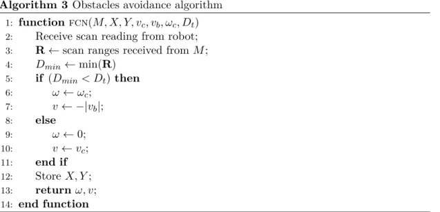
Algorithm 3 Obstacles avoidance algorithm

1: function fcn(M, X, Y, vc, v_b, ωc, Dt)

2: Receive scan reading from robot;

3: R←scan ranges received fromM;

4: Dmin←min(R)

5: if (D_min< D_t) then

6: ω←ω_c;

7: v← −|v_b|;

8: else

9: ω←0;

10: v←vc;

11: end if

12: Store X, Y;

13: return ω, v;

14: end function

Using standard deviations, the Algorithm 5 gives the solution of the problem of repetitive paths (occurs using Algorithm 3) and breaks the repetitive path loop in robot navigation. At the statement28 of the Algorithm5, there is a call to the REVVEL(e) procedure. TheREVVEL(e) procedure is explained in Algorithm4.

Algorithm 4 Procedure to reverse the angular velocity of the robot

1: procedure REVVEL(e)

2: if (e== 1)then

3: ω_c← −ω_c;

4: T₁ ←current time

5: end if

6: T₂ ←current time

7: if (T₂−T₁ > T_d) then

8: e←0;

9: end if

10: end procedure

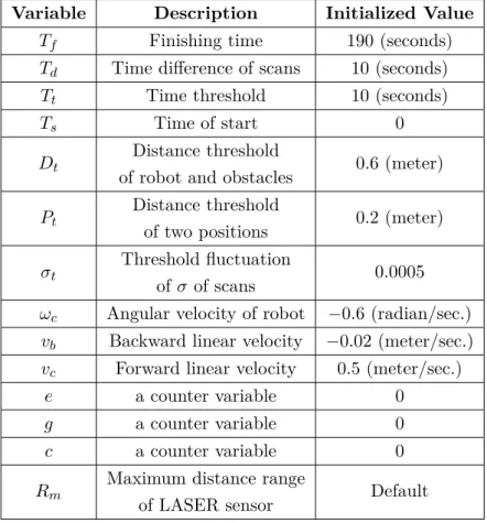
Table1 presents the variables’ descriptions which are taken through Algorithms 3−5.

According to the statement 26 of the Algorithm 5, if the standard deviations, robot positions of the two scans are similar and the time difference between the two scans is larger than a threshold value then this is the re-occurrence of an obstacle.

(21)

Table 1: Variables’ descriptions for the Algorithms3−5.

Variable Description

T_c Current time of the system V Y coordinates vector of positions

when closer obstacles U X coordinates vector of positions

when closer obstacles v Linear velocity of robot Y Y coordinates vector of all positions X X coordinates vector of all positions

ω Angular velocity of robot

S Standard deviations vector of scan ranges

T Vector of scans times

Table 2: Initialization of variables for the Algorithms 3−5.

Variable Description Initialized Value

Tf Finishing time 190 (seconds)

Td Time difference of scans 10 (seconds)

Tt Time threshold 10 (seconds)

Ts Time of start 0

D_t Distance threshold

of robot and obstacles 0.6 (meter) P_t Distance threshold

of two positions 0.2 (meter) σt

Threshold fluctuation

of σ of scans 0.0005

ωc Angular velocity of robot −0.6 (radian/sec.) vb Backward linear velocity −0.02 (meter/sec.) vc Forward linear velocity 0.5 (meter/sec.)

e a counter variable 0

g a counter variable 0

c a counter variable 0

R_m Maximum distance range

of LASER sensor Default

(22)

Algorithm 5 Obstacles recognition and avoidance algorithm

1: Create vectors: Y,S,U,T,V,X;

2: Initialize: D_t, R_m, c, e, g, T_d, T_f, T_t, T_s, P_t, ω_c, σ_t, v_b, v_c; (Definition and initialization of variables can be found in Tables1−2.)

3: while((Tc−Ts)≤Tf) do

4: Read LASER scan from robot;

5: R←Distance range vector received from robot;

6: for j←1 to length (R) do

7: if (R(j) is not defined)then

8: R(j)←R_m;

9: end if

10: end for

11: D_min←min(R);

12: Y(g)←Y coordinate of the robot position;

13: X(g)←X coordinate of the robot position;

14: g←g+ 1; ;

15: if (D_min< D_t) then

16: V(c)←Y coordinate of the robot position;

17: U(c)←X coordinate of the robot position;

18: Compute σ_R using (19);

19: S(c)←σR;

20: T(c)←time at which scan is performed;

21: c←c+ 1;

22: fork←1 to (length (S)−1)do

23: T_d←T(k)−T(c);

24: σ_r←(S(c)−S(k));

25: Dc,k←^p(V(c)−V(k))²+ (U(c)−U(k))² ;

26: if Dc,k< Pt & σr < σt & Td> Tt

then

27: e←e+ 1;

28: Call Procedure REVVEL(e);

29: end if

30: end for

31: ω←ω_c;

32: v← −|v_b|;

33: else

34: ω←0;

35: v←vc;

36: end if

37: Drive the robot using v, ω;

38: end while

(23)

3.3.2 Obstacle recognition and avoidance using two-sample t-test

In Section3.3.1, the Algorithm5 has presented a solution for obstacle recognition and avoidance using the difference of the standard deviations of LASER-scan distance-range- vectors. In Algorithm5, the statement26 is stated as follows:

if(D_c,k< P_t & σ_r < σ_t & T_d> T_t) then

here, the ifcondition composes logical “AND” of three conditions. The second condition (σr< σt) of ifcompares the difference of standard deviations (σr) of two LASER-scan distance-range-vectors with an arbitrary constant value (σ_t). However, setting the value of (σt) is problem specific. Therefore, there is research scope to standardise the condition (σ_r< σ_t).

Various statistical techniques are presented in literature (e.g. [80]). Two independent samples can be compared for similarity on various aspects using t-test [81]. In this section, the comparison of LASER-scan distance-range-vectors is standardised using t-test.

Considering two independent samples (xand y) given in (20) as follows:

x={d_x₁, d_x₂, d_x₃, ..., d_x_n

1}.

y={d_y₁, d_y₂, d_y₃, ..., d_y_n

2}. (20)

Following [83], the statisticst can be defined as follows:

t= d_x−d_y σ_S^q_n¹

1 +_n¹

2

. (21)

where, n₁ and n₂ are the sizes of the x andy samples considered in (20), respectively.

dx and dy are the means of the two samples x and y, respectively. The value of σS is given by (22).

σ_S= v u u u t

1 n1+n2−2





n1

X

i=1

(d_x_i −d_x)²+

n2

X

j=1

(d_y_j−d_y)²



. (22) here,

d_f =n₁+n₂−2. (23)

Application of t-test in obstacle recognition and avoidance:

To apply t-test in obstacle recognition and avoidance, the statements19,24, and26 of the Algorithm 5 can be replaced with the statements given in (24), (25), and (26), respectively.

(24)

Algorithm 6 Procedure to perform t-test on two independent range-vectorsx and y.

1: procedure tTestNk(x, y)

2: n₁ ← size ofx

3: n2 ← size ofy

4: d_f ←n1+n2−2

5: t_c← tabulated value oft corresponding tod_f and level of significance.

6: d_x← _n¹

1

Pn1

i=1d_x_i

7: dy ← _n¹

2

Pn2

j=1dxj

8: Compute σS using equation (22).

9: Compute t using equation (21).

10: if |t|> tc then

11: Return 1

12: else

13: Return 0

14: end if

15: end procedure

S(c)←R (24)

h←tTestNk S(c),S(k) (25)

if ( D_c,k < Pt & h= 0 & T_d> Tt) then (26) where, “tTestNk” is name of the procedure (defined in Algorithm 6). The distance range-vectors, S(c) andS(k), are the two input arguments for a call to the procedure.

The procedure returns “1” if the t-test rejects the null-hypothesis (H₀). On contrary, the procedure returns “0” ifthe t-test accepts the null-hypothesis.

The procedure in Algorithm 6has two input parameters, x andy, pertaining to the input arguments, S(c) and S(k), in it’s call at the modified Algorithm5 using (24) − (26).

(25)

4 New Scientific Results

4.1 Theses Group: Robot navigation with obstacle recognition in unknown static environment having rectangular obstacles

4.1.1 Thesis point-Robot navigation in unknown static environment with obstacle recognition using LASER sensor

The standard deviations of LASER scan distance-range-vectors are suitable for detecting similar obstacle configurations.

Own publication concerned to thethesis point4.1.1: [NK-84, NK-85,NK-86].

4.1.2 Thesis point-Obstacle recognition and avoidance during robot navigation in unknown static environment

In some situations, if similar standard deviations of two LASER scans appears at similar locations and the time difference between the two scans is larger than a threshold value then the path loops can be broken by reversing the angular velocity of the robot.

Own publication concerned to thethesis point4.1.2: [NK-87].

4.1.3 Thesis point-Application of t-test for obstacle recognition and avoidance in robot navigation

Using t-test, similarity of two LASER-scan distance-range-vectors can be checked without comparing the difference of the distance- range-vectors with an arbitrary value. Consequently, the outcome of the t-test can be used for obstacle detection and avoidance.

Own publication concerned to thethesis point4.1.3: [NK-88].

(26)

5 Discussion and Practical Applicability of the Results

In the present time, the robots are getting popular day by day in the scientific, household, and industrial purposes. Importantly, for the mobile robots, the navigation is the key task.

The study presented here has been tested on simulated as well as real robot. Therefore, the research findings of the study can be applied to mobile robots in various fields.

References

[1] A. S. Matveev, A. V. Savkin, M. Hoy, and C. Wang. “8 - Biologically-inspired algorithm for safe navigation of a wheeled robot among moving obstacles”.

In: Safe Robot Navigation Among Moving and Steady Obstacles. Butterworth- Heinemann, 2016, pp. 161–184.

[2] M. Wang, J. Luo, and U. Walter. “A non-linear model predictive controller with obstacle avoidance for a space robot”. In: Advances in Space Research 57.8 (2016). Advances in Asteroid and Space Debris Science and Technology - Part 2, pp. 1737–1746.

[3] Y. Chen and J. Sun. “Distributed optimal control for multi-agent systems with obstacle avoidance”. In:Neurocomputing 173 (2016), pp. 2014–2021.

[4] Jun-Hao Liang and Ching-Hung Lee. “Efficient collision-free path-planning of multiple mobile robots system using efficient artificial bee colony algorithm”.

In:Advances in Engineering Software 79 (2015), pp. 47–56.

[5] J. Lee. “Heterogeneous-ants-based path planner for global path planning of mobile robot applications”. In: International Journal of Control, Automation and Systems 15.4 (Aug. 2017), pp. 1754–1769.

[6] R. Tang and H. Yuan. “Cyclic error correction based q-learning for mobile robots navigation”. In: International Journal of Control, Automation and Systems 15.4 (Aug. 2017), pp. 1790–1798.

[7] A. Narayan, E. Tuci, F. Labrosse, and M. H. M. Alkilabi. “A dynamic colour perception system for autonomous robot navigation on unmarked roads”. In:

Neurocomputing 275 (2018), pp. 2251–2263.

[8] A. Hidalgo-Paniagua, M. A. Vega-Rodríguez, and J. Ferruz. “Applying the MOVNS (multi-objective variable neighborhood search) algorithm to solve the path planning problem in mobile robotics”. In:Expert Systems with Applications 58 (2016), pp. 20–35.

(27)

[9] A. S. Matveev, A. V. Savkin, M. Hoy, and C. Wang. “3 - Survey of algorithms for safe navigation of mobile robots in complex environments”. In: Safe Robot Navigation Among Moving and Steady Obstacles. Butterworth-Heinemann, 2016, pp. 21–49.

[10] A. S. Matveev, A. V. Savkin, M. Hoy, and C. Wang. “4 - Shortest path algorithm for navigation of wheeled mobile robots among steady obstacles”.

In: Safe Robot Navigation Among Moving and Steady Obstacles. Butterworth- Heinemann, 2016, pp. 51–61.

[11] M. Liu, J. Lai, Z. Li, and J. Liu. “An adaptive cubature Kalman filter algorithm for inertial and land-based navigation system”. In: Aerospace Science and Technology 51 (2016), pp. 52–60.

[12] A.L. Amith, A. Singh, H.N. Harsha, N.R. Prasad, and L. Shrinivasan. “Normal Probability and Heuristics based Path Planning and Navigation System for Mapped Roads”. In: Procedia Computer Science89 (2016), pp. 369–377.

[13] M. Ðakulović, M. Čikeš, and I. Petrović. “Efficient Interpolated Path Planning of Mobile Robots based on Occupancy Grid Maps”. In: IFAC Proceedings Volumes 45.22 (2012). 10th IFAC Symposium on Robot Control, pp. 349–354.

[14] J.-Y. Jun, J.-P. Saut, and F. Benamar. “Pose estimation-based path planning for a tracked mobile robot traversing uneven terrains”. In: Robotics and Autonomous Systems 75 (2016), pp. 325–339.

[15] T. T. Mac, C. Copot, D. T. Tran, and R. D. Keyser. “Heuristic approaches in robot path planning: A survey”. In:Robotics and Autonomous Systems 86 (2016), pp. 13–28.

[17] H. Williams, W. N. Browne, and D. A. Carnegie. “Learned Action SLAM: Shar- ing SLAM through learned path planning information between heterogeneous robotic platforms”. In: Applied Soft Computing 50 (2017), pp. 313–326.

[18] G. Younes, D. Asmar, E. Shammas, and J. Zelek. “Keyframe-based monocular SLAM: design, survey, and future directions”. In:Robotics and Autonomous Systems 98 (2017), pp. 67–88.

[19] K. Lenac, A. Kitanov, R. Cupec, and I. Petrović. “Fast planar surface 3D SLAM using LIDAR”. In:Robotics and Autonomous Systems 92 (2017), pp. 197–220.

[20] S. Wen, X. Chen, C. Ma, H.K. Lam, and S. Hua. “The Q -learning Obstacle Avoidance Algorithm Based on EKF-SLAM for NAO Autonomous Walking Under Unknown Environments”. In:Robot. Auton. Syst.72.C (2015), pp. 29–36.

(28)

[21] L. Pfotzer, S. Klemm, A. Roennau, J. M. Zöllner, and R. Dillmann. “Au- tonomous navigation for reconfigurable snake-like robots in challenging, unknown environments”. In:Robotics and Autonomous Systems89 (2017), pp. 123–

135.

[22] A. Elfes. “Using occupancy grids for mobile robot perception and navigation”.

In:Computer 22.6 (June 1989), pp. 46–57.

[23] S. Cossell and J. Guivant. “Concurrent dynamic programming for grid-based problems and its application for real-time path planning”. In: Robotics and Autonomous Systems 62.6 (2014), pp. 737–751.

[24] A. Gil, M. Juliá, and Ò. Reinoso. “Occupancy Grid Based graph-SLAM Using the Distance Transform, SURF Features and SGD”. In:Eng. Appl. Artif. Intell.

40.C (2015), pp. 1–10.

[25] Z. Liu and G. v. Wichert. “Extracting semantic indoor maps from occupancy grids”. In: Robotics and Autonomous Systems 62.5 (2014). Special Issue Se- mantic Perception, Mapping and Exploration, pp. 663–674.

[26] J. Nordh and K. Berntorp. “Extending the Occupancy Grid Concept for Low- Cost Sensor-Based SLAM”. In: IFAC Proceedings Volumes 45.22 (2012). 10th IFAC Symposium on Robot Control, pp. 151–156.

[27] A. M. Santana, K. R.T. Aires, R. M.S. Veras, and A. A.D. Medeiros. “An Approach for 2D Visual Occupancy Grid Map Using Monocular Vision”. In:

Electronic Notes in Theoretical Computer Science 281 (2011). Proceedings of the 2011 Latin American Conference in Informatics (CLEI), pp. 175–191.

[28] L. Dantanarayana, G. Dissanayake, and R. Ranasinge. “C-LOG: A Chamfer distance based algorithm for localisation in occupancy grid-maps”. In: CAAI Transactions on Intelligence Technology 1.3 (2016), pp. 272–284.

[29] P. Schmuck, S. A. Scherer, and A. Zell. “Hybrid Metric-Topological 3D Oc- cupancy Grid Maps for Large-scale Mapping”. In:IFAC-PapersOnLine 49.15 (2016). 9th IFAC Symposium on Intelligent Autonomous Vehicles IAV 2016,

pp. 230–235.

[30] N. Morales, J. Toledo, and L. Acosta. “Path planning using a Multiclass Support Vector Machine”. In:Applied Soft Computing 43 (2016), pp. 498–509.

[31] P. E. Hart, N. J. Nilsson, and B. Raphael. “A Formal Basis for the Heuristic Determination of Minimum Cost Paths”. In: IEEE Transactions on Systems Science and Cybernetics 4.2 (July 1968), pp. 100–107.

(29)

[32] M. M. Deza and E. Deza. Springer-Verlag Berlin Heidelberg, 2009.

[33] E. Hernandez, M. Carreras, and P. Ridao. “A comparison of homotopic path planning algorithms for robotic applications”. In: Robotics and Autonomous Systems 64 (2015), pp. 44–58.

[34] L. E. Kavraki, P. Svestka, J. C. Latombe, and M. H. Overmars. “Probabilistic roadmaps for path planning in high-dimensional configuration spaces”. In:

IEEE Transactions on Robotics and Automation 12.4 (Aug. 1996), pp. 566–580.

[35] R. Geraerts and M. H. Overmars. “Sampling and node adding in probabilistic roadmap planners”. In: Robotics and Autonomous Systems 54.2 (2006).

Intelligent Autonomous Systems, pp. 165–173.

[36] M. R. B. Bahar, A. R. Ghiasi, and H. B. Bahar. “Grid roadmap based ANN corridor search for collision free, path planning”. In: Scientia Iranica 19.6 (2012), pp. 1850–1855.

[37] S. Chaudhuri and V. Koltun. “Smoothed analysis of probabilistic roadmaps”.

In: Computational Geometry 42.8 (2009). Special Issue on the 23rd European Workshop on Computational Geometry, pp. 731–747.

[38] G. Oriolo, S. Panzieri, and A. Turli. “Increasing the connectivity of probabilistic roadmaps via genetic post-processing”. In:IFAC Proceedings Volumes 39.15 (2006). 8th IFAC Symposium on Robot Control, pp. 212–217.

[39] T. Bera, M. S. Bhat, and D. Ghose. “Analysis of Obstacle based Probabilistic RoadMap Method using Geometric Probability”. In: IFAC Proceedings Vol- umes 47.1 (2014). 3rd International Conference on Advances in Control and Optimization of Dynamical Systems (2014), pp. 462–469.

[40] Z. Zheng, Y. Liu, and X. Zhang. “The more obstacle information sharing, the more effective real-time path planning?” In: Knowledge-Based Systems 114 (2016), pp. 36–46.

[41] P. Muñoz, M. D. R-Moreno, and D. F. Barrero. “Unified framework for path- planning and task-planning for autonomous robots”. In: Robotics and Au- tonomous Systems 82 (2016), pp. 1–14.

[42] R. C. Coulter. Implementation of the Pure Pursuit Path Tracking Algorithm.

Tech. rep. CMU-RI-TR-92-01. Pittsburgh, PA: Carnegie Mellon University, Jan. 1992.

(30)

[43] Q. Zhu, J. Hu, W. Cai, and L. Henschen. “A new robot navigation algorithm for dynamic unknown environments based on dynamic path re-computation and an improved scout ant algorithm”. In:Applied Soft Computing 11.8 (2011), pp. 4667–4676.

[44] A. Yorozu and M. Takahashi. “Obstacle avoidance with translational and efficient rotational motion control considering movable gaps and footprint for autonomous mobile robot”. In:International Journal of Control, Automation and Systems 14.5 (Oct. 2016), pp. 1352–1364.

[45] M. Hank and M. Haddad. “A hybrid approach for autonomous navigation of mobile robots in partially-known environments”. In: Robotics and Autonomous Systems 86 (2016), pp. 113–127.

[46] I. Arvanitakis, A. Tzes, and K. Giannousakis. “Mobile Robot Navigation Under Pose Uncertainty in Unknown Environments”. In: IFAC-PapersOnLine 50.1 (2017). 20th IFAC World Congress, pp. 12710–12714.

[47] A. S. Matveev, A. V. Savkin, M. Hoy, and C. Wang. “10 - Seeking a path through the crowd: Robot navigation among unknowingly moving obstacles based on an integrated representation of the environment”. In: Safe Robot Navigation Among Moving and Steady Obstacles. Butterworth-Heinemann, 2016, pp. 229–250.

[48] K. Alisher, K. Alexander, and B. Alexandr. “Control of the Mobile Robots with ROS in Robotics Courses”. In:Procedia Engineering 100 (2015). 25th DAAAM International Symposium on Intelligent Manufacturing and Automation, 2014, pp. 1475–1484.

[49] I. Rodríguez-Fdez, M. Mucientes, and A. Bugarín. “Learning fuzzy controllers in mobile robotics with embedded preprocessing”. In:Applied Soft Computing 26 (2015), pp. 123–142.

[50] Ngangbam Herojit Singh and Khelchandra Thongam. “Mobile Robot Nav- igation Using Fuzzy Logic in Static Environments”. In: Procedia Computer Science 125 (2018). The 6th International Conference on Smart Computing and Communications, pp. 11–17.

[51] T.D. Frank, T.D. Gifford, and S. Chiangga. “Minimalistic model for navigation of mobile robots around obstacles based on complex-number calculus and inspired by human navigation behavior”. In: Mathematics and Computers in Simulation 97 (2014), pp. 108–122.