The Skeleton of Hyperbolic Graphs for Greedy Navigation

(1)

The Skeleton of Hyperbolic Graphs for Greedy Navigation

Zalán Heszberger József B´ıró András Gulyás

Dept. of Telecommunications and Media Informatics, Budapest University of Technology and Economics Budapest, Hungary, biro@tmit.bme.hu

Abstract—Random geometric (hyperbolic) graphs are important modeling tools in analyzing real-world complex networks.

Greedy navigation (routing) is one of the most promising information forwarding mechanisms in complex networks. This paper is dealing with greedy navigability of complex graphs generated by using a metric (hyperbolic) space. Greedy navigability means that every source-destination pairs in the graph can communicate in such a way that every node passes the information towards that neighboring node which is ”closest” to the destination in terms of node coordinates in the metric space. A set of compulsory links in greedy navigable graphs called Greedy Skeleton is identified.

Because the two-dimensional hyperbolic plane (H², also known as the two dimensional Bolyai-Lobachevsky Space [2]) turned out to be extremely useful in modelling and generating real- like networks, we deal with the statistical properties of the Greedy Skeleton when the metric space isH². Some examples of numerical studies and simulation results supporting the analytical formulae are also performed. The significance of the results lies in that every (either artificial or natural) network formation process aiming at greedy navigability must contain this Greedy Skeleton. Furthermore, this could be an important step towards the formal argumentation of the very high greedy navigability of some models observed only experimentally for the time being, and also to analyze equilibrium of greedy network navigation games on H².

Index Terms—Random Hyperbolic Graphs, Greedy Routing, Scale-free Networks

I. INTRODUCTION

A graph embedded in a metric space (nodes of the graphs are labeled with coordinates of the metric space) is said to be greedy navigable (or equivalently said greedy routing is applicable) if greedy path exists between any source- destination pair. Greedy path is a set of consecutive links between a source and a destination, in which the next hop of a node along this path is the neighbor of this node which is closest to the destination in terms of distance measured in the metric space. Clearly, greedy path does not necessarily exist in a graph with an underlying metric space. Informally, if a piece of information (e.g. a packet) arrives at a node, this node should calculate first which of its neighboring nodes is closest to the destination (called also greedy next hop), and then pass the information to this next hop node. In [3] R.

Kleinberg showed in his seminal paper that for each node of an arbitrary graph a virtual coordinate in the hyperbolic plane can be assigned, and greedy routing can be performed with

Thanks OTKA FK17 123957, KH18 129589, K17 124171 for funding.

Heszberger Zal´an is also supperted by MTA Bolyai J´anos Research Grant and UNKP-19-4 Bolyai+ Research Grant.

respect to these virtual coordinates. The assignment is based on his fundamental theorem that every connected finite graph has a greedy embedding in the hyperbolic plane. Nevertheless, this theorem does not provide that this embedding has the desirable properties of low congestion (the number of distinct pairs s, t whose greedy route uses a given node v) and low stretch (the ratio of the number of hops on a greedy route to the number of hops on the shortest route between the same pair of nodes)

In what follows we expose that a skeleton (a set of links in the graph) must exist in every 100% greedy navigable graph. Let a node ube supposed to reach a node v through a greedy path. Let also be the v−centered ball with d(u, v) radius considered. If there is no other node connected to v within this ball, then the (u, v) directed link should exist, otherwise u can not reach v in a greedy manner. In other words,uwill be the closest node tov. Eventually, for all nodes these directed links can be identified, we call them together the Greedy Skeleton. Every node in such a skeleton has only one incoming link (every node has one closest neighbour).

From this it immediately follows that the average degree of the Greedy Skeleton is1. (This could be a good checking point when the degree distribution is derived). A node can have more than one outgoing links (a node can act as a closest node of more than one other nodes).

II. THE SKELETON OF GREEDY NAVIGABLE HYPERBOLIC RANDOM GRAPHS ONH²

A very simple and appealing model using H² as metric space is introduced in [4] for generating scale-free graph, which is as follows: First, place N points (nodes) on a hyperbolic disk with radius R on H², with generating their polar coordinates (r, φ) according to the following density functions¹ on the whole disk

ρ(r) = αsinh(r)

cosh(αR)−1 , ρ(φ) = 1

2π , (1)

where α≥ 1/2 is a parameter controlling the heterogeneity of the layout. If α = 1, the nodes are distributed uniformly over the hyperbolic disk because the area element at coordinates(r, φ)isdA= sinh(r)dr dφ. Next, for every node pair

1Note, that the desired node scattering is achieved in simulations by placing nodesuat polar coordinatesru= (1/α) arccosh{1 + [cosh(αR)−1]U}

andφu= 2πU whereU for eachuis a random number drawn from the uniform distribution on[0,1].

(2)

u, v establish a link between them, if they are not farther than R from each other, i.e. d(u, v) ≤ R, where d(u, v) is the hyperbolic distance betweenu, v onH². This link generation process can also be viewed that for every nodeu, au-centered circle is drawn with radius R, then every point within this circle is connected to u.²

The distance calculation onH²by polar coordinates can be performed by the hyperbolic law of cosine:

cosh(d_uv) = cosh(r_u) cosh(r_v)−sinh(r_u) sinh(r_v) cos(φ) (2) whereru,rv are the radial coordinates of nodesu,vandφis the difference of their angle coordinates.

Now, similarly to the previous discussion, one can identify the greedy skeleton of any greedy navigable graph generated on H² in the following way: Recall that the link (u, v) is contained in GS if and only if the d(u, v)-disk centered at v does not contain any node other than u(see Fig. 1). This means that u cannot reach v by greedy routing through any other nodes thenv, and so a link must exist towardsvto keep greedy navigability of the graph. Note again, that the in-degree of each node in GS will be exactly one.

In the next section, we analyze the statistical properties of GS.

O v

u T_u,v

Fig. 1. An edge in theGS

III. STATISTICAL PROPERTIES OFGS

A. The expected out degree and degree distribution of GS for uniform node density (α= 1)

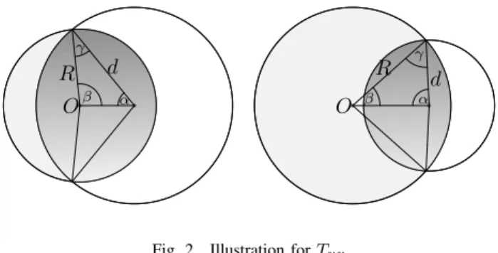
Because the area Tuv of the intersection of the R-disk and the d(u, v)-disk at origin v plays central role in the statistical properties of GS, first we give an approximation for this. An acceptable approximation for Tuv is as follows:

T_uv is apparently equals to 2π(coshd_uv −1)(≈ πe^duv² for not so small d_uv) when the d_uv−disk is completely inside the R−disk. On contrary, if R−r_v < d(u, v) (there is real intersection) then much less evidently Tuv is approximately Tuv≈4e^duv² e^R−²^rv. In Fig. III-A two characteristic cases are depicted when there is real intersection of the duv-disk and the R-disk. Let the polar coordinates of node v be (rv, φv),

2It can also be interpreted that the link establishment rule is a Heaviside step function ond(u, v)asH(R−d(u, v)). In [4] a continuous relaxation ofHis also presented, nevertheless, in this paper we follow the model using H.

and of nodeube(ru, φu). Letφ=|φu−φv|. The areaTuv is the function ofru,rv,φ, andR, and can be calculated as the sum of the two circle sectors with angle 2α, radius duv and angle 2β radius R, and minus the area of the two triangles with anglesα, β, γ. That is

Tuv= 2β(cosh(R)−1)+2α(cosh(duv)−1)−2 (π−α−β−γ) . (3) where the angles and duv are given by the hyperbolic law of cosines, however, here the following simpler approximations are used (which are accurate enough for largerru andduv):

duv≈R+rv+ 2 lnβ

2 ⇒β≈2e^duv² ⁻^R+rv² (4) R≈d_uv+r_v+ 2 lnα

2 ⇒α≈2e⁻^duv² ⁺^R−rv² . (5) Applying (3) with neglecting the triangle areas, and using cosh(R) − 1 ≈ e^R/2, cosh(duv) − 1 ≈ ^e^duv₂ we get T_uv≈4e^duv² e^R−rv² . In summary:

T_uv≈

( πe^d^uv , if 0d_uv< R−r_v 4e^duv² e^R−²^rv , if duv> R−rv .

(6) The expected out-degree as the function of ru can be expressed by the integral:

k_out(r_u) = (N−1) Z

R−disk

TR−Tuv

T_R

^N−2

dT ≈

≈δ Z R

0

Z 2π

0

e^−T^uv^δdφsinh(r_v)dr_v , (7) where Tuv (see Fig. 1) is the area of the intersection of the R-disk and the d(u, v)-disk at origin v andδ=N/T_R is the density of the points (T_R denotes the area of the R-disk).

O O ^β

γ

α

R d

β γ

α

R d

Fig. 2. Illustration forTuv

These approximations are illustrated in Fig. 3 for R= 12, r_v= 6andr_v= 8. Solid lines are the exact T_uv calculations based on (3) and exact computations of angles. Note that there is a sharp change on logarithmic scale between theduv-slope andduv/2-slope aroundR−rv. The dashed lines are theTuv

approximations whenduv> R−rv.

The joint asymptotic expansion of the double integral with respect to rv andφ reveals that the dominant terms will be those in which duv > R−rv. Hence, considering the first integral byφas

δ Z 2π

0

e^−δT^uvdφ . (8)

(3)

2 4 6 8 10 12 10

100 1000 10⁴

duv

Tuv

rv=8 rv=6

Fig. 3. Tuv≈4e^duv² e^R−rv² when there are real intersections (that is when d(u, v)>6and4, respectively).

can be approximated when Tuv is substituted by its approximation, that is by

δ Z 2π

0

e^−δ4e

duv 2 e^R−rv2

dφ . (9)

Applying the approximation e^duv² ≈ e^ru+rv²

q1−cosφ

2 the

integral can be approximated as δ

Z 2π

0

e^−δ4e

duv 2 e^R−rv2

dφ≈2πδ(I(0, x)−S(0, x))≈e⁻^R+ru² (10) where x= 4δe^R+ru² and the last wave due to that I(0, x)− S(0, x) (difference of the BesselI and the modified Struve functions) quickly tends to ²_πx⁻¹. Now the second integration by rv gives the expected degree approximation in the frame topology, that is

k_out,GS(r_u)≈ Z R

0

e⁻^R+ru² sinh(r_v)dr_v= e⁻^R+ru² (cosh(R)−1)≈ 1

2e^R²e⁻^ru² . (11) The quality of this approximation can be checked with the followings. The average in-degree in the frame topology is exactly 1, therefore the average out-degree should also be 1, that is

¯kout,GS = Z R

0

kout,GS(ru) sinh(r_u)

cosh(R)−1dru≈ 1

3(3 +e^−2R−4e^−R/2)≈1 . (12) Let us recall that in case of uniform distribution of points on anR−disk of the hyperbolic plane, the density of the radial coordinates of the points is

ρ(r) = sinhr

coshR−1 (13)

Note that the expected degree of nodeuis exponential in the radial coordinate r_u as in [4]. Because of this and the fact

that equilibrium graph of NNG is also sparse [1] the degree distribution can be calculated in the same way as in [4] :

P(k) = Z R

0

g(k, k_out(r_u))ρ(r_u)dr_u= 1 2

Γ(k−2,¹₂)

k! (14)

where g(k, kout(ru)) is the conditional distribution of the degree of a node with radial coordinateu, and it is Poissonian with mean kout(ru) in case of sparse graphs. It can also be shown that for largerk

P(k)≈ 1

2k³ . (15)

The direct derivation of the complement cumulant degree distribution fromP(k)seems to be intangible, however, from its approximation it can be computed as

F(k)¯ ≈1− Z 1

2k³dk+C

(16) where the constant C is 1, and k ≥ ¹₂ (in order to have distribution function), that is

F(k)¯ ≈ ¯k²

4 k⁻² , k≥1

2 . (17)

It is interesting to show that this approximation can also be obtained as the exact ccdf of the conditional expected node degrees kout(ru). This approximation can be computed as

F¯(k)≈ Z ru(k)

r=0

ρ(r)dr≈e^r^u^(k)−R (18) where ru(k) is the inverse function of kout(ru, R) w.r.t. ru, i.e.

ru(k) =R−2 ln (2k) . (19) Applying this one can obtain the same before as

F(k)¯ ≈ ¯k²

4 k⁻² , k≥1 2

k .¯ (20)

Note that the average degree can also be computed as Z ∞

k=¹₂

k∂(1−F¯(k))

∂k

= 1 (21)

and it is indeed 1.

We have studied the quality of the approximations above also by extensive numerical investigations and eventually found that the exponential decay of the expected degree of nodes (kout(ru)) is extremely good approximation of the numerically evaluated expected degree function for a wide range of node densityδ.

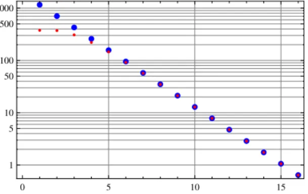
This is illustrated by the following examples. First consider the setupR= 16.5,n= 10000. In this case δ= 2.17·10⁻⁴. Fig. 4 shows how the expected degree decay is matching the exponential decay. One can observe that for larger values of r_uthe coincidence is very good, for smaller values ofr_uthere are larger errors of the approximation.

To quantify this observation, note that 99.9% of points have r_u>10(that is in case of uniformly distributed points on the R(=16.5)-disk, only about 10 points of the 10000 is inside

(4)

0 5 10 15 1

5 10 50 100 500 1000

Fig. 4. Comparison of the exponential decay (C(R)e⁻^ru² , larger blue dots) and the numerically evaluated exact decay (smaller red dots) of the expected degree in the function ofru,R= 16.5,n= 10000.

the disk with radius 10). If we consider the relative errors of the matching one can reveal that for ru > 10 it is smaller than 0.15%, that is for 99.9% of points the expected degree approximation has smaller than 0.15% relative error, as shown by Fig. 5. To increase the number of points ton= 30000and n = 50000 (δ = 6.54·10⁻⁴, δ = 1.08·10⁻³), the relative error is increasing, especially for smaller values ofru, but still for 99.9% of the points the relative error smaller than 0.25%

and 1%, respectively. If we dramatically decrease the node- density, for examplen= 500, the relative errors also increase (compared to the n = 10000 case), however, it still remains under 0.2% for 99.9% of the points.

10 12 14 16

-0.005 -0.004 -0.003 -0.002 -0.001

Fig. 5. Relative error of matching the exponential decay in the function of ru,R= 16.5,n= 10000.

B. The expected out degree and degree distribution of GS for quasi-uniform node density

The radial coordinate density in case of quasi-uniform node density is

ρ(r, α) := αsinh(αr)

cosh(αR)−1 ≈αe^α(r−R) (22) while the angle density remains uniform (_2π¹ ) over the range [1,2π]. Given a point pair (u, v), first we determine the probability p(r_u, α) that the u → v link exists, then based on this the average out degreek(r_u, α)ofuis calculated, and finally F¯(k, α)is also given.

The probabilityp(ru, α)is equal to that none of the remain- ingN−2points fall in the intersection of thev-centeredduv

circle and theR-disk. Let us denote byp1the probability that a point whose coordinates generated by randomly according to the densities above falls inside the intersection. Using p1

the probability p(ru, α) can be calculated and approximated as

p(ru, α) = (1−p1)^N−2≈e^{−N p}¹ (23) The calculation of p1 can be performed by using the node density function in the following way [4]

p1=

Z max(0,d−rv)

0

ρ(r, α)dr+ 1 2π

Z min(R,d+r_v)

|d−rv|

ρ(r, α)2θ(r)dr (24) where

θ(r) = arccoscoshrvcoshr−coshd

sinhrvsinhr . (25) In [4] a useful approximation is presented for quite similar integrals, based on which one can write

p1≈ 4e¹²^(d−R−r^v⁾α

π(−1 + 2α) (26)

for 0.5< α≤1 .

Now the expected out-degree ofucan be written as kout(ru, α)≈ N

2π Z R

0

Z 2π

0

e^{−N p}¹dφρ(rv)drv . (27) Using the approximation ofp1andcosh(d/2)≈e^ru+rv² sin^φ₂ one can formulate

Z 2π

0

e^{−N p}¹dφ≈ Z 2π

0

e^−x^sin^φ²dφ≈2π(I(0, x)−S(0, x))≈ 4 x (28) where

x= 4N π

α

2α−1e^ru²^−R . (29) Note, that x does not depend on rv, therefore the second integration byrv results

k_out(r_u, α)≈ N 2π

4 x

Z R

0

ρ(r_v, α)dr_v =2α−1

2α e^R²e⁻^ru² . (30) Note, that for α= 1 we get back the result for the uniform density case.

Now the (approximation of the) complement cumulative distribution functionF¯(k)can be derived as,

F¯(k) = Z r_u(k)

0

ρ(r, α)dr≈e^α(r^u^(k)−R)=

1−_2α¹ k

^2α

(31) wherer_u(k)is the inverse function ofk_out(r_u).

Here we note that further investigations are needed for deriving analytical formulae for the case0< α≤0.5.

(5)

C. Comparing analytical and simulation results

For comparing the analytical formula and simulation results of the degree distribution of GS, 20 random graphs have been generated each with5000nodes distributed uniformly (α= 1) on a hyperbolic disk with radius R= 15. For each graph the pdf of node degrees is generated and ”averaged” them over the20graphs. Fig 6 shows the results. One can observe good matching for lower degrees, however, in this simulation setup nodes having larger degree than 20 are very rare resulting less reliable statistics for this region.

1 2 5 10 20 50 100

10^-⁴ 0.001 0.01 0.1 1

k

FHkL

Fig. 6. CCDF of the node degrees, analytical formula (continuous line) and the simulation results on a log-log plot.N= 5000,R= 15.

IV. CONCLUSION

We have presented the Greedy Skeleton as a set of mandatory links in every100% greedy navigable graphs. Statistical properties of GS of greedy navigable graphs generated by the metric spaceH²have also been performed. As the main result of this paper, it has been shown that the expected degree of a node in the Greedy Skeleton is proportional to exp(−₂^r) (where r is the radial coordinate of the node in H²) and the degree distribution of the Greedy Skeleton is scale-free that is proportional to k⁻³. Numerical examples and simulation results highlighted the accuracy of the analytical formulae.

REFERENCES

[1] M. Boguna. Class of correlated random networks with hidden variables.

Physical Review E, 68:1–13, 2003.

[2] J. Bolyai. APPENDIX - The Theory of Space (with Introduction, Comments and Addenda by F. Karteszi). North-Holland, 1987.

[3] R. Kleinberg. Geographic Routing Using Hyperbolic Space. InProc. of IEEE Infocom 2007, volume 3, pages 1902 – 1909. IEEE, 2007.

[4] F. Papadopoulos, D. Krioukov, M. Bogua, and A. Vahdat. Greedy forwarding in dynamic scale-free networks embedded in hyperbolic metric spaces. InProc. of IEEE Infocom, pages 1–9. IEEE, 2010.

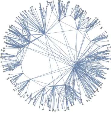
Fig. 7. The full graphN= 350,R= 10to include the mandatory links for navigation. Note that for the ease of illustration, hyperbolic polar coordinates used as Euclidean ones, however, the link establishment is in full accordance of the hyperbolic distance calculation.

Fig. 8. Skeleton necessary for 100% greedy navigable graphs, N = 350, R= 10.