A survey on the global optimization problem using Kruskal–Wallis test
Viliam Ďuriš, Anna Tirpáková
Department of Mathematics
Constantine The Philosopher University in Nitra Tr. A. Hlinku 1, 949 74 Nitra, Slovakia
vduris@ukf.sk atirpakova@ukf.sk Submitted: April 1, 2020
Accepted: May 26, 2020 Published online: June 3, 2020
Abstract
The article deals with experimental comparison and verification of stochas- tic algorithms for global optimization while searching the global optimum in dimensions3and 4of selected testing functions in Matlab computing envi- ronment. To draw a comparison, we took the algorithms Controlled Random Search, Differential Evolution that we created for this test and implemented in Matlab, and fminsearch function which is directly built in Matlab. The basic quantities to compare algorithms were time complexity while searching the considered area and reliability of finding the global optimum of the1st De Jong function, Rosenbrock’s saddle, Ackley’s function and Griewangk’s func- tion. The time complexity of the algorithms was determined by the number of test function evaluations during the global optimum search and we analysed the results of the experiment using the “Kruskal–Wallis test” non-parametric method.
Keywords: global optimization; test functions; simplex; population; Con- trolled Random Search; Differential Evolution; fminsearch; Matlab, Kruskal–
Wallis test
MSC:90C26, 62G09
doi: https://doi.org/10.33039/ami.2020.05.004 url: https://ami.uni-eszterhazy.hu
281
1. Introduction
In mathematics, we often solve a problem that we characterize as finding a mini- mum value of an examined function (so-called global optimization) 𝑓: 𝐷→𝑅 on a specific set 𝐷 ⊆𝑅𝑑, 𝑑 ∈ 𝑁. This minimum value (global minimum or global optimum) is one or more points from the smallest functional value set 𝐷, that is a set {𝑥′∈𝐷:𝑓(𝑥′)≤𝑓(𝑥) ∀𝑥∈𝐷} [8]. From mathematical analysis, we know the procedure for finding the extreme of a function when𝑑= 2and there are the first and second function derivatives. However, finding a general solution to the problem formulated this way is very difficult (or even impossible) for any 𝑑 or if the function considered is multimodal or not differentiable [3]. Any determinis- tic algorithm addressing the generally formulated problem of global optimization is exponentially complex [2]. That is why we use the so-called randomly working (stochastic) algorithms to find a solution to this task, which, although not capable of finding a solution, are capable of finding a satisfactory solution to the problem within a reasonable time. Thus, for the same input problem, such an algorithm performs several different calculations and we aim to create conditions for the al- gorithm so that we reduce the probability of incorrect calculation as much as pos- sible. Today, the use of stochastic algorithms, especially of the evolutionary type, is very successful in seeking global optimization functions [4]. Those are simple models of Darwin’s evolutionary theory of populations development usingselection (the strongest individuals are more likely to survive),crossing (from two or more individuals new individuals with combined parental properties will emerge) and mutation (accidental modification of information that an individual bears); to cre- ate a population with better properties. For some classes of evolution algorithms, the truly best “individuals” of the population are approaching the global optimum.
Experimental verification and comparison of algorithms on test functions offer us an insight into the performance and behavior of the used global optimization algorithms. Based on this, we can then decide which algorithm is most efficient and usable under the given conditions when solving practical tasks. The most basic test functions include the 1st De Jong function, Rosenbrock’s saddle (2nd De Jong function), Ackley’s function and Griewangk’s function. Matlab source code of these functions can be found in [12].
In the Matlab environment, there are several implemented optimization func- tions, of which the fminsearchfunction [6] is very important. The fminsearch function serves for finding a global minimum of the function of multiple variables.
The variables of the function, the global minimum of which we are looking for, are entered into the vector and, also, we specify the so-called start vector𝑥0, from which the search for the minimum will start. The start vector 𝑥0 must be suffi- ciently close to the global minimum (not necessarily in unimodal functions only), because different estimates of the start vector may result in different local minima being found instead of the global one. Since the algorithm fminsearch is based on the so-called simplex method [9], it may happen that the solution will not be found at all. Otherwise, thefminsearchfunction returns the vector𝑥, that is the point
at which the global minimum of the given function is located.
Some optimization parameters for global minimum search can be specified in options structure using the functionoptimset[7]. Then the generic call command of thefminsearchfunction has the form
[x, fval, exitflag, output] = fminsearch(fun, x0, options),
where funis a string that records a given mathematical function,𝑥0 start vector, search setupoptions, xis the resulting vector of the global minimum,fvalfunc- tional value at𝑥,exitflagis a value, which specifies the type of search termination and output is a structure that contains the necessary optimization information (al- gorithm used, number of function evaluations, number of iterations).
For each algorithm, we need to distinguish four types of search termination.
Type 1 is the correct completion of the algorithm when it is found (sufficiently close) to the global minimum, type 2 means that the algorithm is completed by reaching the maximum allowed number of iterations (although it converts to a global minimum), type 3 is an early convergence (the algorithm has completed searches in the local minimum) and type 4 means that browsing is completed by reaching the maximum allowed number of iterations, but no close point to the minimum has been found.
In order to determine the type of algorithm termination for the fminsearch function, it is possible to use the nestedfuncCountelement of theoutputstructure (which gives the number of function evaluations). You can also find out how to complete by using theexitflagelement.
TheControlled Random Search (CRS) algorithm [11] works with a population of 𝑁 points in space 𝐷, from which a new point 𝑦 is generated with the so-called simplex reflex. Simplex 𝑆 ={𝑥1, 𝑥2, . . . , 𝑥𝑑+1}is a set of randomly selected 𝑑+ 1 space𝐷 points. In simplex, we find the point𝑥ℎ= max𝑥∈𝑆𝑓(𝑥)with the highest functional value and, as the worst of simplex, we remove it. To the remaining 𝑑 points, we find their center of gravity
𝑔= 1 2
∑︁
𝑥∈𝑆
(𝑥−𝑥ℎ).
Reflexion means a point overturning𝑥ℎaround the center of gravity𝑔 to obtain a point
𝑦=𝑔+ (𝑔−𝑥ℎ) = 2𝑔−𝑥ℎ.
The simplest variant of the reflection algorithm can then be entered as a function in Matlab as follows: [12]
Reflection algorithm 1: function [y] = reflex(P) 2: N = length(P(:, 1)) 3: d = length(P(1, :)) – 1 4: v = random_simplex(N, d + 1) 5: S = P(v, :)
6: [x, id] = max(S(:, d + 1)) 7: x = S(id, 1:d)
8: S(id, :) = [ ] 9: S(:, d + 1) = [ ] 10: g = mean(S) 11: y = 2*g−x
where a random selection of a set𝑆 is provided by the function
Random selection algorithm
1: function[res] = random_simplex(N, j);
2: v = 1:N;
3: res = [ ];
4: fori = 1:j
5: index = fix(rand(1) * length(v)) + 1;
6: res(end + 1) = v(index);
7: v(index) = [ ];
8: end
If the𝑓(𝑦)< 𝑓(𝑥ℎ), the point𝑦of the population replaces the point𝑥ℎand we continue to do so. In case that𝑓(𝑦)≥𝑓(𝑥ℎ), simplex is reduced. By replacing the worst points of the population, this is concentrated around the lowest functional point being sought. However, the reflection does not guarantee that the newly generated point 𝑦 will be in the searched area 𝐷. Then, we flip all coordinates 𝑦𝑖 ∈ ⟨/ 𝑎𝑖, 𝑏𝑖⟩, 𝑖 = 1, . . . , 𝑑, and inside of the searched area 𝐷 around the relevant side of the 𝑑−dimensional rectangular parallelepiped 𝐷. The algorithm of the so-called mirroring can be entered as a function in Matlab:
Mirroring algorithm
1: function[res] = mirror(y, a, b);
2: f = find(y < a | y > b);
3: fori = f
4: while(y(i) < a(i) | y(i) > b(i)) 5: ify(i) > b(i)
6: y(i) = 2 * b(i) - y(i);
7: elseif(y(i) < a(i)) 8: y(i) = 2 * a(i) - y(i);
9: end 10: end 11: end 12: res = y;
The algorithm’s source text itself,Controlled Random Search, can be then writ- ten as an m-file crs.min Matlab.
CRS algorithm
1:function[FunEvals, fval, ResType] = crs(N, d, a, b, TolFun, MaxIter, fnear, fname);
2: P = zeros(N, d + 1);
3:fori = 1:N
4: P(i, 1:d) = a + (b - a).* rand(1, d);
5: P(i, d + 1) = feval(fname,(P(i, 1:d)));
6:end
7: [fmax, indmax] = max(P(:, d + 1));
8: [fval, indmin] = min(P(:, d + 1));
9: FunEvals = N;
10:while(fmax - fval > TolFun) & (FunEvals < d * MaxIter) 11: y = reflex(P);
12: y = mirror(y, a, b);
13: fy = feval(fname, y);
14: FunEvals = FunEvals + 1;
15:if(fy < fmax) 16: P(indmax, :) = [y fy];
17: [fmax, indmax] = max(P(:, d + 1));
18: [fval, indmin] = min(P(:, d + 1));
19: end 20:end
21:if fval <= fnear
22: if(fmax - fval) <= TolFun 23: ResType = 1;
24: else 25: ResType = 2;
26: end
27:elseif (fmax - fval) <= TolFun 28: ResType = 3;
29:else
30: ResType = 4;
31:end
The FunEvals variable is the counter of the number of algorithms’ function evaluations. As the previous selection𝑁 of population points results in𝑁 function evaluation, it must be preset to the value𝑁. Line10represents a search termination condition(𝑓𝑚𝑎𝑥−𝑓𝑚𝑖𝑛< 𝜖)∨(𝐹 𝑢𝑛𝐸𝑣𝑎𝑙𝑠 > 𝑀 𝑎𝑥𝐼𝑡𝑒𝑟*𝑑)where𝑑is the dimension of the searched area, 𝑓𝑚𝑎𝑥 is the largest functional value that is located in the searched population,𝑓𝑚𝑖𝑛is the smallest functional value,𝜖is the tolerance of the distance of the largest and smallest functional value, MaxIter*d is the limitation of the maximum number of permitted function evaluations during the execution of the algorithm. For test functions, where the solution to the problem is known in advance, it is sufficient that the best point of the population has a value less than f_near, a value close enough to the global minimum that we pre-set. At the end of the algorithm, we find the type of search termination.
Differential Evolutionis a stochastic algorithm for a heuristic search for a global minimum using evolutionary operators [10], [1]. The Differential Evolution algo- rithm creates a new population 𝑄by gradually creating a point 𝑦 for each point 𝑥𝑖, 𝑖= 1, . . . , 𝑁 of the old population𝑃, and assigning a point with a lower func- tional value to the population𝑄from that pair. The point𝑦is created by crossing the vector 𝑣, where the point 𝑣 is generated from three different points, 𝑟1, 𝑟2, 𝑟3
which are randomly selected from the population 𝑃 and different from the point 𝑥𝑖 of the relationship 𝑣 = 𝑟1+𝐹(𝑟2−𝑟3), where 𝐹 > 0 is the input parameter which can be determined according to different rules and the vector 𝑥𝑖 so that any of its elements 𝑥𝑖𝑗, 𝑖 = 1, . . . , 𝑁, 𝑗 = 1, . . . , 𝑑, is replaced by a value 𝑣𝑗 with probability 𝐶 ∈ ⟨0,1⟩. If no change occurs for 𝑥𝑖𝑗 or for 𝐶 = 0 one randomly selected vector𝑥𝑖 element is replaced. We can see that, compared to the algorithm
Controlled Random Search, Differential Evolutiondoes not replace the worst point in a population but only the worse of a pair of points and thus the Differential Evolution algorithm tends to end searches in a local minimum. On the other hand, however, it converges more slowly with the same end condition. The algorithm for generating a point𝑦 can be entered as a function in Matlab [12]:
Algorithm for generating a point𝑦 1: function[y] = gen(P, F, C, v);
2: N = length(P(:,1));
3: d = length(P(1, :)) -1;
4: y = P(v(1),1:d);
5: re = rand_elem(N,3, v);
6: r1= P(re(1),1:d);
7: r2= P(re(2),1:d);
8: r3= P(re(3),1:d);
9: v = r1+ F * (r2- r3);
10: prob = find(rand(1, d) < C);
11: if(length(prob) ==0) 12: prob =1+ fix(d * rand(1));
13: end
14: y(prob) = v(prob);
Selecting points𝑟1, 𝑟2, 𝑟3from the population 𝑃 provides a function
Algorithm for selecting points𝑟1, 𝑟2, 𝑟3
1: function[res] = rand_elem(N, k, v);
2: c =1N;
3: c(v)=[ ];
4: res = zeros(1, k);
5: fori =1:k
6: index =1+ fix(rand(1) * length(c));
7: res(i) = c(index);
8: c(index) = [ ];
9: end
We construct the source text of the algorithmDifferential Evolutionin the same way as with the algorithm Controlled Random Search as the m-filedifevol.m.
Differential Evolution algorithm 1:function[FunEvals, fval, ResType]
= difevol(N, d, a, b, TolFun, MaxIter, fnear, fname, F, C);
2: P = zeros(N, d +1);
3:fori =1:N
4: P(i, 1:d) = a + (b - a) .* rand(1, d);
5: P(i, d + 1) = feval(fname, (P(i, 1:d)));
6:end
7: fmax = max(P(:, d + 1));
8: [fval, imin] = min(P(:, d + 1));
9: FunEvals = N;
10: Q = P;
11: while(fmax - fval > TolFun) (FunEvals < d * MaxIter) 12: fori = 1:N
13: y = gen(P, F, C, i);
14: fy = feval(fname, y);
15: FunEvals = FunEvals + 1;
16: if(fy < P(i, d + 1)) 17: Q(i, :) = [y fy];
18: end 19: end 20: P = Q;
21: fmax = max(P(:, d + 1));
22: [fval, imin] = min(P(:, d + 1));
23: end
24: iffval <= fnear
25: if(fmax - fval) <= TolFun 26: ResType = 1;
27: else
28: ResType = 2;
29: end
30: elseif(fmax - fval) <= TolFun 31: ResType = 3;
32: else
33: ResType = 4;
34: end
2. Methodology of research and algorithms verifica- tion and comparison
The experiment was carried out at the Faculty of Natural Sciences of Constan- tine the Philosopher University in Nitra during the academic years2018/2019and 2019/2020. A total of 42 students of single branch study of mathematics and students of teaching combined with maths, who selected the subject numerical mathematics, participated in the experiment. The group of students was taught a selected part “global optimization” of the mathematics curriculum with use of Matlab.
The aim of our research was to verify the behavior and efficiency of three selected algorithms in the global optimization problem. We used four known test functions to test the efficiency of each of the three selected algorithms. In the experiment while searching a global optimum, we recorded the number of evaluations of each algorithm used for each of the selected function. When algorithms are compared, tests must be performed under the same conditions. The experiment was realized for two different dimensions𝑑= 3 and 𝑑= 4, the number of times the minimum search is repeated to100, tolerance𝜖to the valueseteps = 1e−7; and the default value MaxIter=10000 for one dimension. The search algorithm ends when the minimum and maximum distance are at the selected value or the maximum number of function evaluations has been reached. Especially for the functionfminsearch, the above end condition is maintained by the code sequence:
Termination condition forfminsearch
1:whilefunc_evals < maxfun && itercount < maxiter
2:ifmax(abs(fv(1)-fv(two2np1))) <= max(tolf,10*eps(fv(1))) &&
3: max(max(abs(v(:,two2np1)-v(:,onesn)))) <= max(tolx,10*eps(max(v(:,1)))) 4:break
5:end
in the part Main algorithm of the source text fminsearch [6]. The func_evals variable is in the role of the variable FunEvals, the maxfun constant in the role of the expression MaxIter*d.
The required limit to the number of algorithm iterations and the tolerance of any point in the population from the local minimum point, but also the necessary tolerance 𝜖 of functional values and the limit to the maximum number of test function evaluations can be adjusted by setting the appropriate parameters of the structure options for thefminsearchfunction.
optimset(’MaxFunEvals’, MaxIter*d, ’MaxIter’, MaxIter*d, ’TolX’, seteps,
’TolFun’, seteps));
The dimension of space to be searched, the space limitations, the number of searches repeated and ensuring that the correct function is linked to the algorithm and the correct file name for storing the necessary records are entered through the formalrun_testparameters that can be run for each global optimization algorithm (depending on the altype parameter). While searching for the global optimum, the function writes the repeat number, the number of function evaluations, the type of algorithm termination, the function value of the minimum found into the filenamesaverestext file.
Algorithm for running the test
1: functionrun_test(fname, filenamesaveres, boundary_interval, repcount, d, algtype);
2: N = 10 * d;
3: a = boundary_interval * ones(1, d);
4: b = -a;
5: MaxIter = 10000;
6: seteps = 1e-7;
7: fnear = 1e-6;
8: fid = fopen(filenamesaveres, ’a’);
9: if(algtype == 3) %fminsearch
10: setval = optimset(’MaxFunEvals’, MaxIter*d, ’MaxIter’, MaxIter*d,
’TolX’, seteps, ’TolFun’, seteps);
11: end
12: fori = 1:repcount 13: i
14: switch(algtype) 15: case1 %crs
16: [FunEvals, fmin, ResType] = crs(N, d, a, b, seteps, MaxIter, fnear, fname);
17: case2 %difevol 18: F = 0.8;
19: C = 0.5;
20: [FunEvals, fmin, ResType] = difevol(N, d, a, b, seteps, MaxIter, fnear, fname, F, C);
21: case3 %fminsearch 22: x = a + (b - a).* rand(1, d);
23: [x, fmin, exitflag, output] = fminsearch(fname, x, setval);
24: FunEvals= output.funcCount;
25: iffmin <= fnear 26: ifFunEvals < MaxIter*d 27: ResType = 1;
28: else
29: ResType = 2;
30: end
31: elseif FunEvals < MaxIter*d
32: ResType = 3;
33: else
34: ResType = 4;
35: end 36: end
37: fprintf(fid, ’%5.0f ’, i);
38: fprintf(fid, ’%10.0f’, FunEvals);
39: fprintf(fid, ’ %1.0f’, ResType);
40: fprintf(fid, ’ %15.4e’, fmin);
41: fprintf(fid, ’%1s\r\n’, ’ ’);
42: end 43: fclose(fid);
Thefminsearchalgorithm has 4 output parameters(x, fmin, exitflag, output).
Thus, in determining the type of algorithm termination for thefminsearchfunc- tion, it is not possible to use the non-existent variablefmax. The disadvantage in the run_testfunction above is solved by using the nested funcCountelement of the output structure, which indicates the number of function evaluations.
We ran therun_test function for each dimension, for each algorithm, and for each test function, so we each time got 100 evaluations of the test function by selected algorithm in selected dimension.
Example of calling the run_test function for the1st De Jong function in dimension4 1: fname = ’dejong’;
2: filenamesaveres = ’dejong.txt’;
3: boundary_interval = -5.12;
4: repcount = 100;
5: d = 4;
6: algtype = 1;
7: run_test(fname, filenamesaveres, boundary_interval, repcount, d, algtype);
For example, program code creates a dejong.txt file with 100 rows and 4 columnsi, FunEvals, ResType, fminfor the1st De Jong function in dimension 4, with the CRS algorithm used. Thus, for all combinations of the algorithm and the test function, we get12files for each dimension, each with100evaluations.
3. Results of the experiment and their statistical analysis
Based on the results of the experiment, we can compare the search time complexity [2] and reliability of the algorithms used. The time complexity of the algorithm is determined by the number of test function evaluations during the search, which ensures comparability of results regardless of the speed of the computer used. We analysed the results of the experiment using selected statistical methods. Since we have been following the influence of two factors −the algorithm and function on the assessment numbers, the possibility to use a two-factor variance analysis in
addition to descriptive statistics was offered for the assessment of the results of the experiment. However, we can only use the variance analysis if the following condi- tions are met: The sample files come from the basic files with normal distributions, the sample files are independent of each other and the variances of the basic files are equal. Given that the observed feature assumptions described above were not met, we used the non-parametric method of Kruskal–Wallis test [5] for the analysis.
Since the Kruskal–Wallis test is a non-parametric analogue to a one-factor analysis, all combinations of the levels of the original two factors were a factor: algorithms and types of functions. In our case, we tested3 algorithms in combination with4 types of functions, so we gained12independent selections (sub-groups) or 12 levels of the factor “algorithm type +function type” in each of the two dimensions.
In the experiment, 100 measurements of the assessment numbers were per- formed in dimension3and4in each of the12selections (so-called sub-groups), i.e.
altogether 1200measurements. The tested problem is formulated as follows. We test a null hypothesis𝐻0: the numbers of evaluations in the12sub-groups created according to the factor levels “algorithm type +function type” are identical as in the alternative hypothesis 𝐻1: The numbers of evaluations in the 12sub−groups created according to the factor levels indicated are not identical (or, at least at a level, they are different). As we have already stated, since the condition of the normal distribution of observed features was not met, we used the Kruskal–Wallis test to test the null hypothesis.
The Kruskal–Wallis test is a non-parametric analogue to one-factor variance analysis, i.e. it allows testing the hypothesis 𝐻0 that 𝑘(𝑘≥3) independent files originate from the same distribution. It is a direct generalization of Wilcoxon signed-rank test in the case k of independent selection files(𝑘≥3).
Let’s mark 𝑛1, 𝑛2, . . . , 𝑛𝑘 the ranges of individual selection files. Let’s pose, 𝑛 =𝑛1+𝑛2+· · ·+𝑛𝑘. Let’s line all𝑛 elements into a non-decreasing sequence and let’s assign its rank to each element. Let’s mark 𝑇𝑖 the sum of the elements ranks of the ith selection file (𝑖= 1,2, . . . , 𝑘). Since 𝑇1+𝑇2+· · ·+𝑇𝑘 = 𝑛(𝑛+1)2 must hold, we can use this relationship to check the calculation of the values of the characteristics𝑇𝑖(𝑖= 1,2, . . . , 𝑘). The test statistics is the statistics
𝐾= 12
𝑛(𝑛+ 1)
∑︁𝑘
𝑖=1
𝑇𝑖2
𝑛𝑖 −3 (𝑛+ 1)
which has asymptotically the 𝜒2-distribution with𝑘−1 degrees of freedom. We reject the null hypothesis 𝐻0 at significance level 𝛼 if 𝐾 ≥ 𝜒2(𝑘−1), where 𝜒2(𝑘−1) is the critical value of the 𝜒2-distribution with 𝑘−1 degrees of free- dom. As the statistics 𝐾 has an asymptotic 𝜒2-distribution, we can only use the above relationship if the selections have a large range(𝑛𝑖≥5, 𝑖= 1,2, . . . , 𝑘), and if 𝑘≥4. For some 𝑖 is𝑛𝑖 <5, or if𝑘 = 3, we compare the test criteria value 𝐾 with the critical value𝐾𝛼of the Kruskal–Wallis test. Critical values𝐾𝛼are listed in the critical values table. The tested hypothesis 𝐻0 is rejected at significance level𝛼if𝐾≥𝐾𝛼.
If identical values occur in the obtained sequence data, that are assigned the average rank, it is necessary to divide the value of the testing criterion 𝐾 by the so−called correction factor. Its value is calculated by the following formula:
𝑓 = 1−
∑︀𝑝 𝑖=1
(︀𝑡3𝑖 −𝑡𝑖)︀
𝑛3−𝑛
where𝑝is the number of classes with the same rank,𝑡𝑖 the number of ranks in the 𝑖−th class. The testing statistics will then have the form
𝐾2=𝐾 𝑓 .
If we reject the tested hypothesis 𝐻0 in favour of the alternative hypothesis 𝐻1, which means that the selections do not come from the same distribution, a question remains unanswered: which selections differ statistically significantly from each other. In the analysis of variance, Duncan test, Tukey method, Scheffe method or Neményi test are used to answer this question. In the Kruskal–Wallis test, Tukey method is most frequently used to test contrasts, which we also briefly describe below.
In the Tukey method, we compare the𝑖−th and the𝑗−th file for each𝑖, 𝑗, where 𝑖, 𝑗 = 1,2, . . . , 𝑘and 𝑖̸=𝑗, according to the following procedure. For each pair of compared files, we calculate average ranks
𝑇¯𝑖= 𝑇𝑖
𝑛𝑖, 𝑇¯𝑗= 𝑇𝑗
𝑛𝑗.
The testing criterion of the null hypothesis𝐻0, that the distributions of the files𝑖 and𝑗 are identical, is the absolute value of the difference in their average rank
𝐷=⃒⃒𝑇¯𝑖−𝑇¯𝑗⃒⃒.
The tested hypothesis𝐻0 is rejected at significance level𝛼, if𝐷 > 𝐶, where 𝐶=
√︃
𝜒2𝛼(𝑘−1)𝑛(𝑛+ 1) 12
(︂1 𝑛𝑖
+ 1 𝑛𝑗
)︂
𝜒2𝛼(𝑘−1)is the critical value of the𝜒2−distribution with𝑘−1degrees of freedom, 𝑘is the number of compared files. In our case, we verified by the Kruskal–Wallis test whether the12 sub-groups produced by the level of the factor “type of algorithm + type of function” statistically significantly differ in the observed feature “the numbers of evaluations”. Therefore𝑘= 12, while𝑛1=𝑛2 =· · ·=𝑛12= 100, 𝑛= 𝑛1+𝑛1+· · ·+𝑛12 = 1200are measured numbers of evaluations. We implemented the Kruskal–Wallis test in program STATISTICA. After entering the input data in the computer output reports, we get the following results for the selected Kruskal–
Wallis test: the testing criterion value 𝐻 and the probability value𝑝.
Dimension 3
We have used the Kruskal–Wallis test to test the null hypothesis𝐻0: the numbers of evaluations in the12sub-groups created according to the factor levels “algorithm type+function type” are identical as in the alternative hypothesis𝐻1: the numbers of evaluations in the12sub-groups created according to the factor levels indicated are not identical (or, at least at a level, they are different).
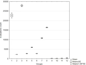
First, we calculated arithmetic averages and standard deviations of the assess- ment numbers (Table 1) and also presented it graphically in Figure 1 in each of the12sub-groups.
Evaluations count
Groups Means N Std. Dev.
1 22709,21 100 7098,061
2 2249,60 100 114,419
3 27863,82 100 3143,617
4 2703,36 100 191,001
5 5980,20 100 328,916
6 2711,70 100 117,233
7 10827,00 100 1327,715
8 16384,20 100 1092,761
9 192,89 100 25,877
10 234,79 100 14,931
11 272,89 100 28,379
12 376,47 100 69,821
All Grps. 7708,84 1200 9504,885
Table 1: Numbers of evaluations in each subgroup in dimension 3
Figure 1: Numbers of evaluations (average values) in each subgroup in dimension3
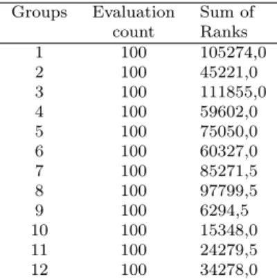
We have calculated the rank sums Table 2, the test criterion value𝐾= 1172.02
and the value 𝑝= 0.000 by the Kruskal–Wallis test in dimension3 for the assess- ment numbers. As the calculated probability value𝑝is less than0.01, we reject the null hypothesis at the significance level𝛼= 0.01, i.e. the difference between the12 sub-groups in dimension3 with respect to the observed feature of the “number of evaluations” is statistically significant.
Groups Evaluation Sum of
count Ranks
1 100 105274,0
2 100 45221,0
3 100 111855,0
4 100 59602,0
5 100 75050,0
6 100 60327,0
7 100 85271,5
8 100 97799,5
9 100 6294,5
10 100 15348,0
11 100 24279,5
12 100 34278,0
Table 2: Kruskal–Wallis test results
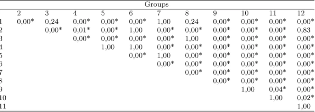
The test confirmed that the individual sub-groups in dimension3 differ statis- tically significantly from each other in relation to the assessment numbers. In the same way, as in dimension2, we have been able to find out by multiple comparisons which groups are statistically significantly different from each other Table3in this case.
Groups
2 3 4 5 6 7 8 9 10 11 12
1 0,00* 1,00 0,00* 0,00* 0,00* 0,00* 1,00 0,00* 0,00* 0,00* 0,00*
2 0,00* 0,22 0,00* 0,14 0,00* 0,00* 0,00* 0,00* 0,00* 1,00
3 0,00* 0,00* 0,00* 0,00* 0,27 0,00* 0,00* 0,00* 0,00*
4 0,11 1,00 0,00* 0,00* 0,00* 0,00* 0,00* 0,00*
5 0,18 1,00 0,00* 0,00* 0,00* 0,00* 0,00*
6 0,00* 0,00* 0,00* 0,00* 0,00* 0,00*
7 0,70 0,00* 0,00* 0,00* 0,00*
8 0,00* 0,00* 0,00* 0,00*
9 1,00 0,02* 0,00*
10 1,00 0,01*
11 1,00
Table 3: Results of Kruskal–Wallis multiple comparison test (𝑝-values)
The Table 3 shows that there is a statistically significant difference in the num- bers of evaluations in dimension3 between sub-group1and sub-group2, between sub-group 1 and sub-groups 4 to 7 and between the sub-group 1 and sub-groups 9 to 12 (probability value𝑝= 0.000). This means that the measured assessment
numbers in sub-group1are statistically significantly different as measured in sub- group 2 and sub-groups 4 to 7 and 9 to 12 (or the assessment numbers between sub-groups 1st and 2nd and between the1st sub-group and sub-groups 4–7 a 9–
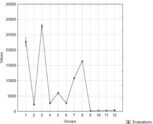
12 are significantly different respectively). In the same way, we can interpret all results in Table 3 marked with a *. We also illustrated the situation graphically (Figure 2).
Figure 2: Numbers of evaluations (average values) in each subgroup in dimension3
Dimension 4
As in previous dimensions, we also tested the statistical significance of differences in the number of evaluations in 12 sub-groups by the Kruskal–Wallis test in di- mension 4. In each of the12 sub-groups of dimension4, we calculated arithmetic averages and standard deviations of the number of evaluations (Table 4) and we also presented the situation graphically in Figure3.
We have calculated the rank sums (Table 5) and the test criterion value𝐾 = 1180.46 and the value 𝑝 = 0.000 by the Kruskal–Wallis test. As the calculated probability value𝑝is as well less than0.01in this case, we reject the null hypoth- esis at the significance level𝛼= 0.01, i.e. the difference between the12sub-groups in dimension 4 with respect to the observed feature “numbers of evaluations” is statistically significant. The Kruskal–Wallis test confirmed that the individual sub-groups in dimension 4 differ statistically significantly from each other in re- lation to the assessment numbers. Subsequently, we have identified by multiple comparisons (Table 6) which groups are statistically significantly different from each other. Table 6 shows that there is a statistically significant difference in the numbers of evaluations in dimension4 between sub-group1and sub-group2. and sub-group 1 and sub-groups 4 to 6 and between the sub-group 1 and sub-groups
Evaluations count
Groups Means N Std. Dev.
1 34741,03 100 3119,75
2 4666,28 100 186,43
3 40000,00 100 0,00
4 5618,71 100 237,65
5 11676,80 100 518,89
6 4992,00 100 160,60
7 22800,00 100 2404,70
8 40000,00 100 0,00
9 298,57 100 57,56
10 379,91 100 44,35
11 439,19 100 61,26
12 609,18 100 129,52
All Grps 13851,81 1200 15432,29
Table 4: Numbers of evaluations in each subgroup in dimension 4
Figure 3: Numbers of evaluations (average values) in each subgroup in dimension4
9 to 12 (probability value𝑝= 0.000). This means that the measured assessment numbers in sub-group 1 in dimension 4 are statistically significantly different as measured in this dimension in sub-groups2,4to6as well as9to12(or the assess- ment numbers between sub-groups1and sub-groups4−7and9−12in dimension 4are significantly different). In the same way, we can interpret all results in Table 6 marked with a*. We also illustrated the situation graphically (Figure 4).
Groups Evaluation Sum of
count Ranks
1 100 105000,0
2 100 49972,5
3 100 105000,0
4 100 65050,0
5 100 75050,0
6 100 50127,5
7 100 85200,0
8 100 105000,0
9 100 5884,5
10 100 16658,5
11 100 23892,5
12 100 33764,5
Table 5: Kruskal–Wallis test results Groups
2 3 4 5 6 7 8 9 10 11 12
1 0,00* 0,24 0,00* 0,00* 0,00* 1,00 0,24 0,00* 0,00* 0,00* 0,00*
2 0,00* 0,01* 0,00* 1,00 0,00* 0,00* 0,00* 0,00* 0,00* 0,83
3 0,00* 0,00* 0,00* 0,00* 1,00 0,00* 0,00* 0,00* 0,00*
4 1,00 1,00 0,00* 0,00* 0,00* 0,00* 0,00* 0,00*
5 0,00* 1,00 0,00* 0,00* 0,00* 0,00* 0,00*
6 0,00* 0,00* 0,00* 0,00* 0,00* 0,00*
7 0,00* 0,00* 0,00* 0,00* 0,00*
8 0,00* 0,00* 0,00* 0,00*
9 1,00 0,04* 0,00*
10 1,00 0,02*
11 1,00
Table 6: Results of Kruskal–Wallis multiple comparison test (𝑝-values)
Figure 4: Numbers of evaluations (average values) in each subgroup in dimension4
4. Conclusion
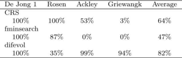
In conclusion, we can summarize based on the results of the experiment that the fminsearchfunction is the fastest algorithm and, on the other hand, the Differ- ential Evolution algorithm is the slowest one. Only type 1 search is considered successful. Then the reliability of finding the global minimum can be characterized as the relative number of type1termination, that is𝑅= 𝑛𝑛1, where𝑛1is the num- ber of type1terminations and𝑛the number of repetitions. The algorithms based on the experiment determine this reliability (in percent) of the global minimum finding (Table 7).
De Jong1 Rosen Ackley Griewangk Average
CRS100% 100% 53% 3% 64%
fminsearch
100% 87% 0% 0% 47%
difevol
100% 35% 99% 94% 82%
Table 7: Reliability of algorithms id dimensions3and4
We can see a considerable difference in the reliability of theDifferential Evolu- tionalgorithm (which is very slow) and algorithmsControlled Random Search and fminsearch. We can say that evolutionary operations mutation, cross-breeding, and selection are a major benefit of reliability for the algorithm. The difference in reliability of the algorithmControlled Random Search andFminsearch can also be considered significant given the number of times the global minimum search and the test functions used are repeated. Furthermore, based on the results of the test, we can say that finding a global minimum of the First De Jong function is simple and almost certain for any algorithm. Finding a global minimum forRosen- brock’s saddle is not easy just for an algorithmDifferential Evolutionthat searches unreliably. From the above-mentioned reliabilities, it can be said that finding the global minimum of theAckley functionandGriewangk’s functionis difficult for the truly fast Fminsearch algorithm implemented in the Matlab environment, which produces great results for the Second De Jong function reliably and quickly. In general, the finding of the global minimum of the Griewangk’s function is least likely in dimensions3and4.
Based on the results of the experiment, we can conclude that by involving math- ematical software to solve global optimization problems, a higher level of knowledge was achieved, a better understanding of various principles and algorithms, and, thus, students better mastered the issue. It is therefore effective and necessary to pay sufficient attention to these methods. Thanks to the use of computer tech- niques in the pedagogical process, everyone can draw into mathematics secrets of global optimization problems. On the basis of the results and theoretical starting points of the work, we have arrived at the following recommendations:
1. lead the students in solving mathematical application tasks in order to best
understand the theoretical starting points of the subject topic
2. use computer technology to increase students’ activity and to provide a suc- cessful motivation to work
3. create suitable, modern and pregnant study material that will enhance the knowledge of students
4. within the cross-subject relations, extend the students’ knowledge from the computer algebra systems
5. involve the use of computer algebra systems into maths teaching for achieving better results
6. effectively use the subject matter from another field within the framework of cross-subject relationships (such as mathematics and informatics).
References
[1] Y. Gao,K. Wang,C. Gao,Y. Shen,T. Li:Application of Differential Evolution Algo- rithm Based on Mixed Penalty Function Screening Criterion in Imbalanced Data Integration Classification, Mathematics 7.12 (2019), p. 1237,
doi:https://doi.org/10.3390/math7121237.
[2] M. R. Garey,D. S. Johnson:Computers and intractability, vol. 174, Freeman San Fran- cisco, 1979.
[3] K. N. Kaipa,D. Ghose:Glowworm swarm optimization: theory, algorithms, and applica- tions, vol. 698, Springer, 2017,
doi:https://doi.org/10.1007/978-3-319-51595-3.
[4] V. Kvasnicka,J. Pospíchal,P. Tino:Evolutionary algorithms, STU Bratislava (2000).
[5] D. Markechová,B. Stehlíková,A. Tirpáková:Statistical Methods and their Applica- tions. FPV UKF in Nitra, 534 p, 2011.
[6] Mathworks:Online documentation, accessed 6th March, 2020, 2020, url:https://www.mathworks.com/help/matlab/ref/fminsearch.html.
[7] Mathworks:Online documentation, accessed 16th March, 2020, 2020, url:https://www.mathworks.com/help/matlab/ref/optimset.html.
[8] S. Míka:Mathematical optimizatio, Plzeň: ZCU Plzeň, 1997.
[9] J. A. Nelder:A Simplex Method for Function Minimization, Computer Journal 7.1 (1964), pp. 308–313.
[10] K. Price,R. M. Storn,J. A. Lampinen:Differential evolution: a practical approach to global optimization, Springer Science & Business Media, 2006.
[11] W. L. Price:A Controlled Random Search Procedure for Global Optimization, Computer Journal 20.4 (1977), pp. 367–370.
[12] J. Tvrdík:Evolutionary algorithms, Ostrava: University of Ostrava, 2010.