ORIGINAL STUDY
Developing a global model for the conversion of zenith wet tropospheric delays to integrated water vapour
Juni Ildikó1 · Rózsa Szabolcs1
Received: 11 January 2018 / Accepted: 28 March 2018 / Published online: 19 April 2018
© Akadémiai Kiadó 2018
Abstract The tropospheric wet delay is a significant systematic error of GNSS position- ing, nevertheless it carries important information to meteorologists. It is closely related to the integrated water vapour that is the upper limit of precipitable water. The zenith wet delay can be converted to the integrated water vapour using a simple conversion factor.
This conversion factor can be determined with the empirical formulae derived from radio- sonde observations. In the past decades, numerous models were derived for this purpose, but all of these models rely on radiosonde observations stemming from a limited area of the globe. Although these models are valid for the area, where the underlying radiosonde observations were measured, there are several examples that these empirical formulae are used to validate GNSS based integrated water vapour estimations all over the globe. Our aim is to create a global model for the conversion of the zenith tropospheric delay to the integrated water vapour for realtime and nearrealtime applications using globally available Numerical Weather Models (NWM). Thus our model takes into consideration the fact that the model parameters strongly depend on the geographical location. 10 years of monthly mean ECMWF (European Center for Medium-Range Weather Forecast) dataset were used for the derivation of the model parameters in a grid with the resolution of 1° × 1°. The empirical coefficients of the developed models depend on two input parameters, namely the geographical location and the surface temperature measured at the station. Thus, the new models can be used for both realtime and near-realtime GNSS meteorological applica- tions. The developed models were validated using 6 years of independent global ECMWF monthly mean analysis datasets (2011–2016). The results showed, that the application of the original models outside the area of the underlying radiosonde data sets can result in a relative systematic error of 7–8% in the estimation of the conversion factor as well as the estimated IWV values.
* Juni Ildikó
juni.ildiko@epito.bme.hu
1 Department of Geodesy and Surveying, Budapest University of Technology and Economics, Muegyetem rkp 3, Budapest 1111, Hungary
Keywords Wet tropospheric delay · Integrated water vapour · Conversion factor · GNSS meteorology
1 Introduction
The Global Navigation Satellite Systems (GNSS) are parts of our everyday life. The tropo- spheric delay is one of the systematic error sources of GNSS that is mostly considered in positioning applications. However, the wet part of the tropospheric delay plays an important role in meteorology, too. Since its value depends on the atmospheric water vapour, it can be converted into integrated water vapour with a simple empirical function. Bevis et al. (1992) and Emardson and Derks (2000) determined such empirical formulae. The previous is derived from 8718 radiosonde observations from the United States, while the latter one is developed from 128,649 European measurements. Since the underlying data sets were obtained from a limited part of the globe, they provide the highest accuracy in these areas.
In the recent years numerous publications were published, in which the aforementioned models were used outside the area, which the underlying data sets were obtained from. (Haase et al. 2003; Igondová and Cibulka 2010). Such an application of these models neglects the geographical variation of model parameters. When radiosonde profiles are available in the study area, a more rigorous approach is to derive local models for this conversion (Mekik and Deniz 2016; Deniz et al. 2016). However, radiosonde observations are not available in many parts of the world to fit the conversion model parameters to the local/regional climate. In these areas usually the model proposed by (Bevis et al. 1992) is used for the conversion, neglecting the climatic dependency of the model parameters.
In this paper another approach is proposed. Since Numerical Weather Models (NWM) pro- vide global datasets of meteorological parameters with a grid resolution of 1° × 1°, these data sets can be used to derive a global model for the conversion of zenith tropospheric wet delays to integrated water vapour. This global model can take into consideration the geographical variations of the model parameters, thus it can provide optimal empirical parameters all over the world.
The developed models are validated using independent global NWM datasets obtained from the past 6 years.
2 The determination of the conversion factor 2.1 The method of Bevis
According to Bevis et al. (1992) the relationship between the integrated water vapour and the wet tropospheric delay can be expressed by a simple conversion factor:
where Q is the conversion factor (kg/m3), IWV corresponds to the integrated water vapour (kg/m2) and ZWD denotes the wet tropospheric delay in the zenith direction (m). The con- version factor is computed in two steps (Bevis et al. 1992). Firstly the mean temperature of the water vapour is calculated with an empirical formula:
(1) Q= IWV
ZWD,
(2) Tm=a0+a1⋅Ts.
The formula denotes a linear relation between these quantities, where Tm is the mean temperature of water vapour (K) and Ts is the surface temperature (K). The offset is a0 = 70.2 K and the slope is a1 = 0.72 that are computed from 2 year dataset consist of 8718 radiosonde observations from the latitude between 27° and 65° of the United States.
Using the following equation the conversion factor can be determined with the mean temperature of the water vapour (Rózsa et al. 2009):
where Rd = 286.9 J/kg/K is the specific gas constant of dry air and Rv = 461.5 J/kg/K denotes the specific gas constant of water vapour, k1 = 0.77604 K/Pa, k2 = 0.64790 K/Pa and k3 = 3776 K2/Pa are empirical constants proposed by Thayer (1974).
2.2 The method of Emardson and Derks
Emardson and Derks (2000) determined the conversion factor directly using a polynomial model of the surface temperature:
where the parameters are computed from 128,649 atmospheric profiles observed between the years 1989–1997 at 38 European radiosonde stations. The parameters are:
a0 = 6.458 m3/kg, a1 = − 1.78 × 10⁻² m3/kg/K, a2 = − 2.2 × 10⁻⁵ m3/kg/K2 and T = 283.49 K.
3 Methodology
The parameters of the showed models are based on observations obtained from a limited area only (United States, Europe), but they are commonly used on other areas of the Earth to estimate integrated water vapour from GNSS observations (Haase et al. 2003; Igondová and Cibulka 2010). Our aim is to derive new models using the upper models that take into consideration the climatic effects. Thus global NWM were used to derive the empirical parameters of Eqs. 2 and 4 for every grid point with a resolution 1° × 1°. In the following parts of the paper, the developed model that follows the approach of Bevis (Eq. 2) will be referred as the ‘Linear model’ while the developed model that follow the approach of Emardson and Derks (Eq. 4) will be referred as the ‘Polynomial model’.
3.1 Meteorological data
The monthly mean solutions of the European Centre for Medium-Range Weather Forecasts (ECMWF) ERA-Interim analysis were used to derive the new global models of the conversion factor. A global grid with the resolution of 1° × 1° for the years of 2001–2010 were retrieved from ECMWF. Temperature, relative humidity and geopotential values on all of the given 37 pressure levels were considered. Afterwards, the water vapour pressure was calculated for
Q= 106 (3) Rv⋅
(−Rd
Rv ⋅k1+k2+ k3
Tm
),
Q= 1 (4)
a0+a1⋅ (
TS−T) +a2⋅
(
TS−T)2,
each level using the given relative humidity and the ambient temperature. Moreover, the geo- potential values were calculated to heights above the Mean Sea Level.
The stratosphere above the troposphere can also cause the error of some centimeters in the tropospheric delay (Rózsa et al. 2012). Since ECMWF models does not cover this area of the atmosphere, these datasets were extended up to the height of 86 km using the International Standard Atmosphere (ISA, ISO Standard 2533,1975).
3.2 Calculating the parameters of the improved models
In order to derive a global grid of model parameters for the Polynomial model, it is neces- sary to calculate the integrated water vapour (IWV) and the zenith wet delay (ZWD) from the NWM, since the conversion factor can be computed for these two quantities according to Eq. 1. Moreover, the calculation of the mean temperature of water vapour for each grid point and epoch is needed to derive the parameters of the Linear model according to Eq. 2. When these quantities are available for all the grid points and all the 120 epochs, then the parameters of the Linear (Eq. 2) and the Polynomial models (Eq. 4) can be determined for the whole global grid as a linear or quadratic regression function of the surface temperature.
3.2.1 Computation of the wet tropospheric delay using the ray‑tracing method The ray-tracing method supposes various layers of the atmosphere that have different mete- orological data (Boehm and Schuh 2003). Applying this method, the path of the satellite beam is traced. The beam starts at a certain elevation angle from the surface of the Earth. Then it refracts continuously at the boundaries of the layers based on the Snell’s law and changes its direction.
The resolution of the data must be increased to calculate the ray-tracing with a sufficient accuracy. The increments of the height is specified as follows (Rocken et al. 2001): between 0–2 km 10 m, between 2–6 km 20 m, between 6–16 km 50 m, between 16–36 km 100 m, between 36–136 km 500 m. These heights are used to interpolate the temperature values lin- early and the air pressure and the water vapour pressure exponentially. These vertically densi- fied meteorological parameters can be used to calculate the wet refractivity of each layer:
where i = 1, 2,…k, where k is the number of the atmospheric layer, Nwi is the wet refrac- tivity in the given layer (−), Mw= 0.0180152 kg/mol denotes the molar mass of the water vapour, Md= 0.0289644 kg/mol is the molar mass of dry air, T corresponds to the tempera- ture (K) and e is the water vapour pressure (hPa).
The next step is to determine the distance that the ray travels in the respective layer. The total wet tropospheric delay can be calculated as a sum of the products of the length of the refracted beam and the wet refractivity in every layer:
where si the length of the refracted beam in the i-th layer (m).
(5) Nwi =
( k2−k1⋅
Mw Md
)
⋅ ei Ti +k3⋅
ei Ti2,
(6) ZWD=
∑k−1 i=1
si⋅
Nwi+Nwi+1
2 ,
3.2.2 The calculation of the integrated water vapour
The integrated water vapour depends on the air pressure, the temperature, the relative humidity and the local gravity acceleration. Firstly, the mixing ratio is calculated using the vertically interpolated meteorological data (WMO 2008):
where pi (hPa) is the air pressure and MRi (−) denotes the mixing ratio that expresses the ratio between the mass of the water vapour and the mass of the dry air in the given layer.
The integrated water vapour can be computed in the specific layers:
where g (m/s2) is the local gravity acceleration that depends on the latitude. The total IWV can be calculated as the sum of the IWV in the specific layers.
3.2.3 The mean temperature of water vapour
The mean temperature of water vapour plays a role in the derivation of the Linear model.
Firstly the water vapour density can be calculated:
where ρv (kg/m3) describes the water vapour density. Using this, the mean temperature of water vapour can be expressed (Askne and Nordius 1987):
where hmax (m) is the height of the topmost level of our meteorological data sets, namely 86,000 m.
4 Model developments 4.1 Linear model
Linear model expresses a linear relation between the mean temperature of the water vapour (Tm) and the surface temperature (Ts) according to Eq. 2. Altogether 120 values for the mean temperature of water vapour and of the surface temperature are computed for the grid with a global resolution of 1° × 1° using ECMWF monthly mean data of (7) MRi=621.98⋅ei
pi−ei ,
(8) IWVi=1
g⋅(
pi−1−pi)
⋅
MRi−1+MRi
20 ,
(9) IWV =
∑k−1
i
IWVi
(10) 𝜌v= e⋅100
Rv⋅T,
(11) Tm=
∫hhmax
0
𝜌vdz
∫hhmax
0 𝜌v Tdz
,
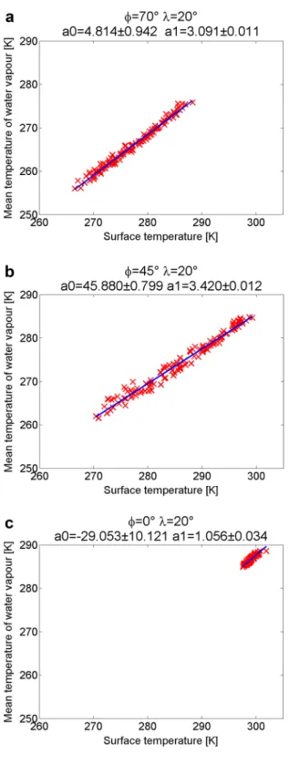
10 years. To compute the parameters of Eq. 2 a linear regression line was fitted to the 120 Tm − Ts data pairs for every grid point. The uncertainty of the fitting is the largest at the Equator, due to the low variability of both of the variables (Fig. 1).
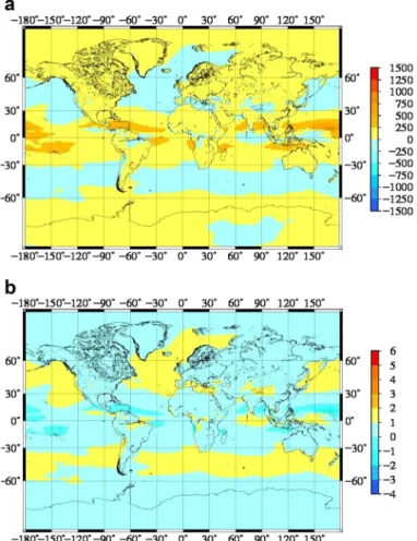
The a0 and a1 parameters of the improved model (Eq. 2) are available in a global grid with resolution 1° × 1° (Fig. 2). The figure shows that the model parameters differ from the parameters proposed by Bevis et al. (1992) on large areas of the continents.
The largest differences can be observed along the Equator, and in high mountains like the Andes and the Himalayas.
Based on the derived global grid of model parameters, the conversion factor between the zenith wet delay and the integrated water vapour can be calculated for any geographical location on the Earth. Firstly, the mean temperature of the water vapour is calculated using the derived parameters and the surface temperature by Eq. 2 for the four neighbouring grid points. Afterwards the conversion factor is computed for all the four grid points using Eq. 3. Finally, the conversion factor is calculated at the speci- fied geographical location using bilinear interpolation. For real-time and near realtime GNSS meteorological applications, the zenith wet delay is estimated from the GNSS observations. The estimated zenith delays can be easily converted to integrated water vapour using the conversion factor provided by the Linear model at the location of the GNSS station using Eq. 1. This method takes into consideration the effect of climate on the conversion parameters.
4.2 The polynomial model
Polynomial model parameters were derived based on the method proposed by Emard- son and Derks (2000). In this case, the conversion factor can be expressed as a direct function of the surface temperature and the mean of the surface temperatures (Eq. 4).
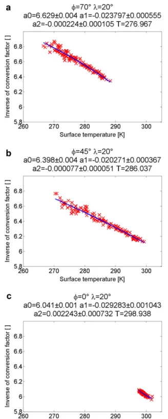
The relationship between the inverse of the conversion factor, the surface temperature and the mean of the surface temperatures can be represented by a second order pol- ynom. The wet tropospheric delay and the integrated water vapour are calculated using ECMWF monthly mean data for 10 years with the resolution of 1° × 1°. Afterwards the multiplicative inverse of the conversion factor is determined by the reciprocal of Eq. 1.
There are 120 differences between the surface temperature and the mean of the sur- face temperatures related with 120 multiplicative inverse of conversion factor values in every grid point. Finally, a second order polynomial is fitted to the differences and the multiplicative inverse of the conversion factors in every grid point (Fig. 3).
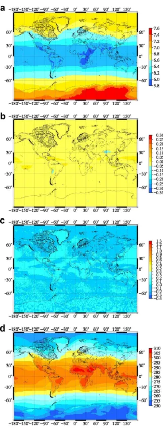
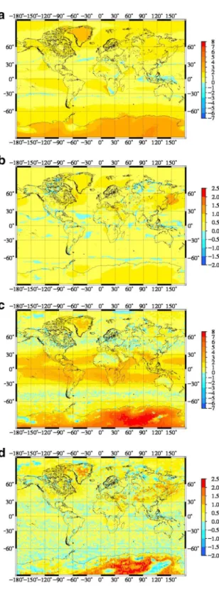
The four parameters of the Polynomial model (a0, a1, a2 and T ) are given in a global grid with the resolution of 1° × 1° (Fig. 4). The derived parameters show a significant difference with respect to the original Emardson and Derks model parameters around the Equator.
For GNSS meteorology applications, the conversion factor can be calculated using a similar approach proposed for the Linear model. Based on the specified location of the GNSS station, the conversion factor can be calculated for the four adjacent grid points using Eq. (4) as a function of surface temperature. Applying bilinear interpola- tion using these four conversion factor values, the conversion factor at the location of the station can be calculated. Afterwards, the ZWD estimated from the GNSS observa- tions can be easily converted to IWV using this conversion factor value.
Fig. 1 Linear model—line fitting to 120 Tm– Ts data along longitude 20° at latitude 70°, 45°
and 0° and the calculated a0 (K), a1 (−) parameters
5 Validation of the improved models
In order to validate the derived models globally, ECMWF Numerical Weather Models were obtained for the period of 2011–2016. This enabled us to validate our results using independent meteorological data sets from the ones used for the derivation of the models.
The reference values of the zenith wet delays, the integrated water vapour and the mean temperature of the water vapour were obtained using the same methodology as given in Sect. 3.
The validation of the models are done in two ways. The first validation tests examined the newly developed models from the perspective of the temporal stability of the model parameters. In this case, the model parameters were estimated using the independent data set obtained from 2011 to 2016, and the conversion factor values provided by these model parameters were compared to the original values given by Bevis et al. (1992) and the val- ues of the globally available Linear model. A similar comparison is done for the Polyno- mial model and the original Emardson and Derks model.
Fig. 2 The derived a0 and a1 parameters of the Linear model with resolution 1° × 1°. These can be com- pared to the parameters of Bevis model where a0 = 70.2 K
Fig. 3 Polynomial model—pol- ynom fitting to 120 1/Q − Ts data along longitude 20° at latitude 70°, 45° and 0° and the calcu- lated a0 (m3/kg), a1 (m3/kg/K), a2 (m3/kg/K2)
Fig. 4 The derived a a0, b a1, c a2 and d T parameters of the Polynomial model with resolution 1° × 1°. These can be compared to the parameters of Emardson–Derks model
In the second validation test, the NWM data sets were used to derive the ZWD and the IWV as reference values. Afterwards, the ZWD values were converted to estimated IWV values using the conversion factors obtained from the Linear and Polynomial models, and the estimated IWV values were compared to the reference values of IWV calculated by numerically integrating the atmospheric profiles at each grid points using the NWM. In the following sections the results of the validation tests are discussed.
5.1 Validation of temporal stability of model parameters
In this validation test, the mean temperature of water vapour, the zenith wet tropospheric delay and the integrated water vapour is calculated using 6 years of ECMWF monthly mean NWM data. The parameters of the Reference Linear model were determined with 72 Tm − Ts values in every grid point (Eq. 2) and the parameters of the Reference-Polynomial model were calculated with 72 1/Q − Ts data (Eq. 4) over the whole 1° × 1° grid. After- wards the conversion factors were determined with the parameters and surface tempera- ture using the Reference-Linear model (Eqs. 2, 3) and for the Reference-Polynomial model (Eq. 4), too.
In order to validate results the conversion factor values of Linear/Polynomial model and Reference-Linear/Reference-Polynomial model were compared. The validation was done using the relative bias and the relative standard deviation of the residuals of the conversion factors. To quantify the relative bias and standard deviation, the following formulae were used:
where Qmean% (%), Qstd% (%), QR (kg/m3) denotes the conversion factor of the reference model, QB,ED (kg/m3) is the conversion factor of the original Bevis or Emardson and Derks model and QL,P (kg/m3) expresses the conversion factor of the improved Linear/Polynomial model (Fig. 5). The positive values mean the improved Linear/Polynomial model gives bet- ter result than Bevis or the Emardson and Derks model.
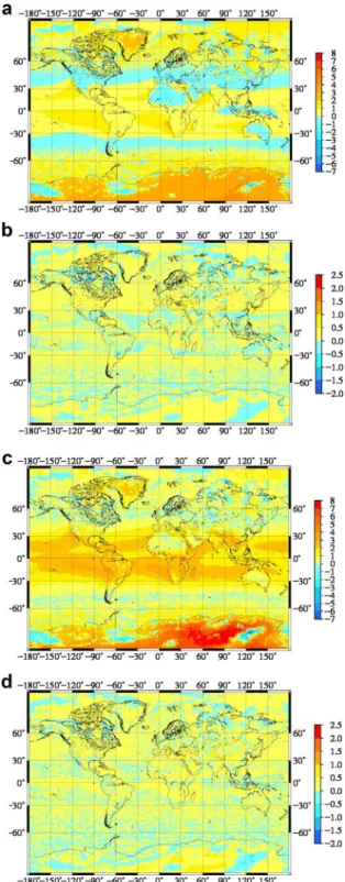
Analysis of Qmean% (%) at the Linear model shows almost everywhere slightly better results (1–2%) than the original Bevis model. There are bigger improvements close to the poles, the values of Qmean% reach 3–5% (Fig. 5a). The relative bias of the Polynomial model shows larger improvements around the Equator compared to the original Emardson and Derks model (Qmean% is between 1 and 4%). Though there are two bands around the lati- tude of approximately 45° on both the northern and the southern hemispheres, where the Polynomial model gives slightly worse results (approximately 1% in terms of relative bias) (Fig. 5c), this is most likely the effect the underlying data sets. Since the original Emard- son and Derks model was derived from radiosonde data sets from this region, the small negative relative bias can be explained by the higher accuracy of the radiosonde profiles obtained from in situ observations with respect to the NWM.
Qstd% are mostly somewhat better (0.5–1.5%) for the Linear model (Fig. 5b). Qstd%
map for the Polynomial model shows mixed results. In many regions of the globe the Qmean%= (12)
||
|(mean(
QR−QB,ED)|
||−|
||(mean(
QR−QL,P)|
||
meanQR ⋅100
Qstd%= (13)
||
|(std(
QR−QB,ED)|
||−|
||(std(
QR−QL,P)|
||
meanQR ⋅100
Fig. 5 First approach of valida- tion a, c Qmean% at linear/poly- nomial (%) (Eq. 12) b, d Qstd%
at linear/polynomial model (%), (Eq. 13)
improvement is in the order of 0.5–2.5%, while in other places a slight deterioration can be observed (0.5–1%) (Fig. 5d). However, the largest improvement can be observed over the Antarctica in terms of uncertainties.
The mean values of the Qmean% and Qstd% values for both the Linear and Polynomial models can be found in Table 1. The values show that both of the models provide an improvement in the order of 1–1.5% globally in terms of bias.
It must be noted that this approach examines systematic error only, since the two linear and polynomial models derived using different underlying data sets are compared. The ran- dom error values are eliminated with the line/polynom fitting during the derivation of the reference models. The second validation test aims at the consideration of both the system- atic and random effects.
5.2 Validating the performance of the developed conversion factor models for GNSS meteorology applications
The wet tropospheric delay and the integrated water vapour values are calculated using 6 years of ECMWF monthly mean analysis data in this test. The conversion factor can be expressed as a function of these quantities (Eq. 1) for a global grid that can be directly used as reference values for validating the derived Linear and Polynomial models. In order to carry out the validation, the developed models are used to estimate the conversion factor for each grid points. The residuals are formed as the difference of the conversion factors obtained from the NWM data used for the validation and the conversion factor estimated by either the Linear or the Polynomial models. Finally, Eqs. 12 and 13 were used to calcu- late both the Qmean% and Qstd% relative improvement coefficients for the bias and standard deviation of the residuals at each grid point (Fig. 6).
The Qmean% for the Linear model shows improvement around the Equator (1–2%) (Fig. 6a). For the latitude band between N35° and N55° latitudes the improved Linear model gives worse results than the original Bevis model (1–2%). The largest improvements can be observed in Greenland and the Antarctica. The Polynomial model shows very simi- lar results to the first approach in terms of Qmean% (Fig. 6c). It must be noted that the area of the slightly worse performance coincides with the geographical location of the underlying data sets used for the derivation of the original Bevis and the Emardson and Derks mod- els. Thus it can be stated, that the conversion factor models derived from local or regional radiosonde observations perform slightly better in the appropriate regions compared to the models obtained from global NWM. However it is also visible on the figures that both the developed Linear and Polynomial models perform better outside these latitude bands.
Qstd% shows mixed results. In some cases a slight improvement (0.5–1%) can be observed while in other cases slightly worse (0.5–1%) results are obtained in terms of standard deviations (Fig. 6b, d).
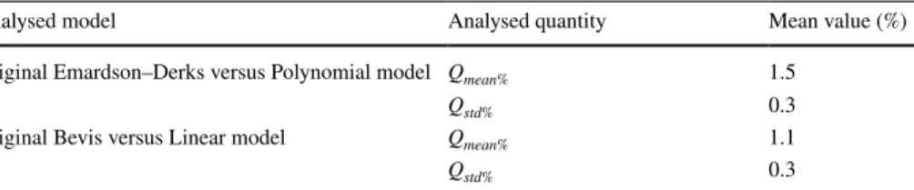
Table 1 The mean of Qmean% and Qstd% values at first approach-line/polynom fitting
Analysed model Analysed quantity Mean value (%)
Original Emardson–Derks versus Polynomial model Qmean% 1.5
Qstd% 0.3
Original Bevis versus Linear model Qmean% 1.1
Qstd% 0.3
Fig. 6 Second approach of validation a, c Qmean% at linear/
polynomial (%) (Eq. 12) b, d Qstd% at linear/polynomial model (%), (Eq. 13)
The global mean values of the Qmean% and Qstd% values for both the Linear and Polyno- mial models can be found in Table 2. These results show that a slight improvement could be achieved in the order of 1–1.5% in terms of bias while no improvement can be observed in terms of standard deviations. Since the former term reflects the systematic error while the latter the random error, one can state that the systematic error of the conversion factor models could be decreased with our approach. In other words, the developed model shows a slightly smaller systematic bias in the estimation of the conversion factors used for the calculation of IWV from ZWD estimated using GNSS observations.
6 Summary and conclusions
Based on empirical formulae derived by Bevis et al. (1992) and Emardson and Derks (2000) two new models were derived for the estimation of the conversion factor between the ZWD and the IWV for GNSS meteorological applications. These models are called the Linear and the Polynomial models. The new models take the climatic effects into consid- eration, since the model parameters were derived from ECMWF monthly mean analysis data between 2001 and 2010 for a global grid with the resolution of 1° × 1°. The conversion factors were validated using 6 years of independent global ECMWF monthly mean analy- sis datasets (2011–2016).
The results show that the newly derived models perform better than the original ones in many regions of the world in terms of systematic bias. The only area, where the original models perform better coincidences with the area of the underlying radiosonde data sets of these models, suggests that radiosonde observations are still more suitable for deriving locally or regionally fitted conversion factor models compared to the NWM data. How- ever radiosonde stations are not homogeneously distributed over the whole globe, thus this approach can not be applied globally.
The proposed approach of this study can fill these gaps, since our models perform bet- ter in other regions of the world compared to the original models derived from radiosonde observations. The results showed that the application of the original models proposed by Bevis et al. and Emardson and Derks outside the area of the underlying radiosonde data sets can result in a relative systematic error of 7–8% in the estimation of the conversion factor as well as the estimated IWV values. Thus it is more advantageous to use the devel- oped models in regions where no conversion factor models were derived using local radio- sonde observations.
The parameters of both the Linear and the Polynomial models are available for down- loading at the website: http://gpsme t.agt.bme.hu/zwd2i wv for free.
It must also be noted that the atmospheric products of the Global Geodetic Observing System (Nafisi et al. 2012) contain a global grid of the mean temperature of water vapour
Table 2 The mean of Qmean% and Qstd% values at second approach-IWV/ZWD method
Analysed model Analysed quantity Mean value (%)
Original Emardson–Derks versus Polynomial model Qmean% 1.4
Qstd% 0.1
Original Bevis versus Linear model Qmean% 0.7
Qstd% 0.0
(Tm) that can be used to calculate the conversion factor directly using Eq. (3). However these results are published using NWM analysis only, therefore they are not available for realtime and near realtime applications. The models proposed by this study can fill this gap, since our models does not rely on the availability of current NWM and Tm values, thus both of the models can be used for both realtime and near realtime applications.
References
Askne J, Nordius H (1987) Estimation of tropospheric delay for microwaves from surface weather data.
Radio Sci 22(3):379–386
Bevis M, Businger S, Herring TA, Rocken C, Anthes A, Ware R (1992) GPS meteorology: remote sensing of atmospheric water vapour using the global positioning system. J Geophys Res 97:15787–15801.
https ://doi.org/10.1029/92JD0 1517
Boehm J, Schuh H (2003) Vienna mapping functions. 16. Working meeting on European VLBI for geodesy and astrometry, pp 131–143
Deniz I, Mekik C, Gurbuz G (2016) Spherical harmonics functions modelling of meteorological parameters in PWV estimation. In: Conference paper ‘living planet symposium 2016’, Prague, Czech Republic, 9–13 May 2016
Emardson TR, Derks HJP (2000) On the relation between the wet delay and the integrated precipitable water vapour in the European atmosphere. Meteorol Appl 7:61–68. https ://doi.org/10.1017/S1350 48270 00013 77
Haase J, Ge M, Vedel H, Calais E (2003) Accuracy and variability of GPS tropospheric delay measure- ments of water vapor in the western Mediterranean. J Appl Meteorol 42(11):1547–1568. https ://doi.
org/10.1175/1520-0450(2003)042%3C154 7:AAVOG T%3E2.0.CO;2
Igondová M, Cibulka D (2010) Precipitable water vapour and zenith total delay time series and models over Slovakia and vicinity. Contrib Geophys Geodesy 40(4):299–312. https ://doi.org/10.2478/v1012 6-010-0012-6
ISO 2533: 1975 standard, Standard Atmosphere (1975)
Mekik C, Deniz I (2016) Modelling and validation of the weighted mean temperature for Turkey. Meteorol Appl 24(1):92–100. https ://doi.org/10.1002/met.1608
Nafisi V, Madzak M, Böhm J, Ardalan A, Schuh H (2012) Ray-traced tropospheric delays in VLBI analysis.
Radio Sci 47:2. https ://doi.org/10.1029/2011R S0049 18
Rocken C, Sokolovskiy S, Johnson JM, Hunt D (2001) Improved mapping of tropospheric delays. J Atmos Ocean Technol 18:1205–1213. https ://doi.org/10.1175/1520-0426(2001)018%3C120 5:IMOTD
%3E2.0.CO;2
Rózsa SZ, Dombai F, Németh P, Ablonczy D (2009) Integrált vízgőztartalom becslése GPS adatok alapján Geomatikai Közlemények XII. pp 187–196
Rózsa SZ, Weidinger T, Gyöngyösi AZ, Kenyeres A (2012) The role of GNSS infrastructure in the monitor- ing of atmospheric water vapor. Q J Hung Meteorol Serv 116:1–20
Thayer GD (1974) An improved equation for the radio refractive index of air. Radio Sci 9:803–807 World Meteorological Organization (WMO) (2008) Guide to meteorological instruments and methods of
observation. WMO-No. 8