Folyamatok analízise és szintézise bizonytalan paraméterek mellett

(1)

PhD Dissertation

ANALYSIS AND SYNTHESIS OF PROCESSES WITH UNCERTAIN PARAMETERS

Éva König

Supervisor:

Dr. Botond Bertók

University of Pannonia Faculty of Information Technology Doctoral School Information Science

2020

DOI:10.18136/PE.2020.751

(2)

ANALYSIS AND SYNTHESIS OF PROCESSES WITH UNCERTAIN PARAMETERS

Thesis for obtaining a PhD degree in the Doctoral School of Information Science of the University of Pannonia

in the branch of Information Sciences Written by Éva König

Supervisor: Dr. Botond Bertók

propose acceptance (yes / no) ……….

(supervisor/s)

The PhD-candidate has achieved ... % in the comprehensive exam,

Veszprém, ……….

(Chairman of the Examination Committee) As reviewer, I propose acceptance of the thesis:

Name of Reviewer: …... …... yes / no

……….

(reviewer) Name of Reviewer: …... …... yes / no

……….

(reviewer)

The PhD-candidate has achieved …...% at the public discussion.

Veszprém, ……….

(Chairman of the Committee)

The grade of the PhD Diploma …... (…….. %) Veszprém,

……….

(Chairman of UDHC)

(3)

Acknowledgement

First of all, I would like to thank my supervisor Dr. Botond Bertók for leading my research all along in the past 8 years by his knowledge and ideas and by introducing me to highly qualied scientists. I am also grateful to Professor Heriberto Cabezas for introducing me to the eld of Information Theory and for leading our brand new research regarding systems' resilience.

Without their knowledge, ideas and guidance I would have never been capable of accomplishing this work.

I thank Dr. Csaba Fábián for giving me strong base knowledge in stochastic programming and stochastic optimization.

I highly appreciate the support of Audrey L. Mayer in the systems' resilience research, she has provided crucial information regarding the Isle Royale National Park's ecosystem and regarding ecosystems in general.

I would like to thank Dr Zoltán Süle for his great help in the P-graph related approaches.

I am grateful to my former and present colleagues who are always there for helping me.

Finally and most importantly, I would like to thank my family and friends for continuously believing in me, celebrating smaller milestones with me and helping me getting up after every defeat and getting through hopeless situations.

iv

(6)

Abstract

One of the key components in industry and market supply is the freight transportation, besides the expanding market relies on the eciency of shipments even more. In transportation, uncertainty cannot be neglected, e.g., trac or navigability of rivers, seas, or weather conditions at airports and their stochastic nature can aect contracts between a rm and a transport company. Analysis of contracts' conditions is essential, whether they have short or medium term validity, e.g., the rst costs less while the latter can oer more exibility. Medium term scenario analysis can be formulated as a two-stage decision problem, which are typically managed by methods applying decision trees. Since realistic problems are complex enough to result in a decision tree with enormous size, application of these kind of methods is limited in practice.

In this thesis there is a computer aided algorithmic method presented based on P-graph framework, which is able to implicitly involve and enumerate all feasible scenarios instead of explicitly enumerate the possibilities, and the problem formulation is still kept compact and transparent. For supporting long term decisions regarding complex systems, the direct calculation of the resilience of a system's current regime has the highest importance. Concerning ecosystems, resilience (the system's resistance to disturbances) is a key concern for managing human impacts on them and managing their risk of collapse. Approaches applying statistics or information theory have conrmed utility in identifying regime boundaries. In this thesis, Fisher information is used to establish the limits of the resilience of a dynamic regime of a predator-prey system. The importance of this technique lays in the focus of the approach. Previous studies using Fisher information focused on detecting whether a regime change has occurred, whereas here the attention is on determining how much an ecological system can vary its properties without a regime change occurring. The theory and the method are illustrated with simple two species systems; rst it is applied to a predatory-prey model system and then to a 60-year wolf- moose population dataset from Isle Royale National Park in Michigan, USA. The resilience boundaries and the operating range of a system's parameters are assessed without a regime change from entirely new criteria for Fisher information, oriented towards regime stability. The approach provides possibility to use system measurements to determine the shape and depth of the stability cup as dened by the broader resilience concept.

(7)

Kivonat

Az ipar és a piaci kínálat egyik kulcseleme a teherfuvarozás, emellett a b®vül® piac még inkább tá- maszkodik a szállítmányozás hatékonyságára. A szállítással kapcsolatban nem lehet gyelmen kívül hagy- ni a bizonytalanságot, például a forgalmat, a folyók, tengerek vagy a repül®terek id®járási körülményeit vagy a hajózhatóságot; ezek sztochasztikus jellege befolyásolhatja a vállalkozás és a szállítmányozó cég közötti szerz®déseket. A szerz®dések feltételeinek elemzése elengedhetetlen, függetlenül attól, hogy azok rövid vagy középtávon érvényesek, például az el®bbi költsége alacsonyabb, míg az utóbbi na- gyobb rugalmasságot nyújthat. A középtávú forgatókönyv elemzás megfogalmazható kétlépcs®s dön- tési problémaként, amelyet általában döntési fákat alkalmazó módszerekkel közelítenek meg. Mivel a valós problémák elég bonyolultak ahhoz, hogy hatalmas méret¶ döntési fát eredményezzenek, az ilyen módszerek alkalmazhatósága a gyakorlatban korlátozott. Ebben a dolgozatban számítógépes al- goritmikus módszer kerül bemutatásra, amely a P-gráf keretrendszeren alapul, és amely képes im- plicit módon bevonni és leszámlálni az összes lehetséges forgatókönyvet, ahelyett, hogy explicit módon sorolná fel az összes lehet®séget, amellett, hogy a probléma megfogalmazása továbbra is kompakt és átlátható marad. A komplex rendszerekkel kapcsolatos hosszú távú döntések támogatása szempontjából a legfontosabb a rendszer aktuális állapotának ellenálló képessége és annak közvetlen kiszámítása. Az ökoszisztémák vonatkozásában az ellenálló képesség (a rendszer zavarokkal szembeni ellenálló képessége) kulcsfontosságú az ®ket érint® emberi hatások és a rendszerösszeomlás kockázatának kezelése szempont- jából. A statisztikát vagy az információelméletet alkalmazó megközelítések igazolták a rezsimhatárok azonosításának fontosságát. Ebben a dolgozatban a Fisher információ kerül alkalmazásra a zsákmány- ragadozó dinamikus rendszer ellenálló képesség korlátainak meghatározására. Ennek a technikának je- lent®sége a megközelítésben rejlik. A Fisher információt alkalmazó korábbi tanulmányok arra irányultak, hogy észleljék a rendszerek közötti váltásokat, míg itt a gyelem annak meghatározására irányul, hogy egy ökológiai rendszer tulajdonságai, paraméterei mennyiben változhatnak anélkül, hogy rendszervál- tozás következne be. Az elméletet és a módszert egyszer¶, két fajból álló rendszer szemlélteti; el®ször egy ragadozó-zsákmány modell rendszer, majd egy 60 éves farkas-jávorszarvas populáció-adatállomány, az Egyesült Államok Michigan állambeli Isle Royale Nemzeti Parkból. Az ellenálló képesség határait és a rendszer paramétereinek m¶ködési tartományát a módszer úgy képes megbecsülni a Fisher-információ teljesen új, adatokra vonatkozó kritériumai alapján, hogy a rendszer közben nem változik meg, azaz a rendszer stabilitására koncentrál. Ezzel a megközelítéssel lehet®vé válik az ellenállóképesség tágabb megfogalmazása szerinti csésze mélységének és szélességének meghatározása a rendszer mér®számainak felhasználásával.

vi

(8)

Abstracto

Uno de los componentes clave en la industria y el suministro del mercado es el transporte de carga, además el mercado en expansión depende aún más de la eciencia de los envíos. En el transporte, no se puede descuidar la incertidumbre. Por ejemplo, el tráco o la navegabilidad de ríos, mares o las condiciones climáticas en los aeropuertos y su naturaleza estocástica puede afectar los contratos entre una empresa y una empresa de transporte. El análisis de las condiciones de los contratos es esencial, ya sea que tengan validez a corto o mediano plazo. Por ejemplo, el primero cuesta menos mientras que el segundo puede ofrecer más exibilidad. El análisis de escenarios a mediano plazo se puede formular como un problema de decisión en dos etapas, que generalmente se manejan mediante métodos que aplican árboles de decisiónes. Dado que los problemas realistas son lo sucientemente complejos como para generar un árbol de decisiónes con un tamaño enorme, la aplicación de este tipo de métodos es limitada en la práctica. En esta tesis sepresenta un método algorítmico asistido por computadora basado en el marco de P-graph. Este es capaz de involucrar y enumerar implícitamente todos los escenarios factibles en lugar de enumerar explícitamente las posibilidades, y la formulación del problema aún se mantiene compacta y transparente. Para soportar decisiones a largo plazo con respecto a sistemas complejos, el cálculo directo de la resistencia del régimen actual de un sistema tiene la mayor importancia. Con respecto a los ecosistemas, la resiliencia (la resistencia del sistema a las perturbaciones) es una interés clave para manejar los impactos humanos sobre ellos y manejar su riesgo de colapso. Los enfoques que aplican estadísticas o teoría de la información han conrmado su utilidad para identicar los límites del régimen. En esta tesis, la información de Fisher se utiliza para establecer los límites de la resistencia de un régimen dinámico de un ecosistema predador-presa. La importancia de esta técnica radica en el enfoque del método. Estudios previos que utilizaron información de Fisher se centraron en detectar si se produjo un cambio de régimen, mientras que aquí la atención está en determinar cuánto puede variar un sistema ecológico sus propiedades sin que ocurra un cambio de régimen. La teoría y el método se ilustran con sistemas simples de dos especies; primero se aplica a un sistema modelo de presas-predadoras y luego a un conjunto de datos de población de lobos y alces de 60 años del Parque Nacional Isle Royale en Michigan, EE.UU. Los límites de resiliencia y el rango operativo de los parámetros de un sistema se evalúan sin un cambio de régimen de criterios completamente nuevos para la información de Fisher, orientados hacia la estabilidad del régimen. El método brinda la posibilidad de utilizar mediciones del sistema para determinar la forma y la profundidad de la copa de estabilidad tal como se dene en el concepto de resiliencia más amplio.

(9)

Chapter 1

Introduction

There are several ways to support decision making depending on the decision maker, the type of decision, the system itself that is aected by the certain decision, or the time frame that species the decision. In this thesis, the focus is on two dierent methods that are able to support decisions practically with strong mathematical bases. The rst presented method is a multi- stage optimization approach considering uncertainty assisting short- and midterm decisions for companies. The second technique presented in this work is much more relevant for long-term maintenance of huge and complex systems by using the Fisher information and providing the possibility to the direct calculation of the system's resilience, the ability of the system to persist within a certain regime in the presence of disturbances. In other words, the rst method is for optimal design of the structure of complex systems, while the other approach is able to dene the dynamic systems' limits and boundaries within the system can remain in a certain regime.

The thesis is written in passive voice but the new results are highlighted as I have actively worked on them all along my PhD studies.

In the following sections, the aim of this thesis is determined, then comes the brief overview of the background and relevant literature for both above introduced methods for decision support.

In the succeeding chapters, the new techniques are described in detail, rst the multi-stage stochastic optimization method and then the approach for calculating systems' resilience using Fisher information. Each method is illustrated by a representative example. After summarizing the presented work, the new scientic results and the related publications are highlighted in separate chapters.

1.1 Aim

Optimal processes are essential in all sectors of business and industry so that a company can stay competitive and ecient in the market. However, uncertainty cannot be neglected when speaking of making optimal decisions. Several robust and reliable process network optimization algorithms and software have been developed and implemented on the basis of the P-graph framework in

1

(10)

the last three decades, e.g., Algorithm SSG [33], Algorithm ABB [34], Software PNS-Studio [9].

The approach based on the P-graph framework is capable of generating mathematical model automatically, and providing the n-best networks for process synthesis. All the steps involved are mathematically proven, such as comprehensive superstructure generation, mathematical model construction, optimization and the solution interpretation. An optimization problem with uncertain parameters can be solved by the P-graph framework in several ways depending on which parameters are uncertain or how the unpredictability is taken into consideration.

If the uncertainty is considered only in the available ow of resources, there is a P-graph based technique that is able to provide the optimal structure with minimal cost and expected reliability.

For this method, the original algorithms have been extended to consider the reliability of the raw materials' availability and to guarantee the predened level of reliability for the overall process design. Another P-graph based approach is capable of identifying the least sensitive among all the feasible solution structures, if the cost or the available ow of the resources, the activity cost, and the required ow of the product can be stochastic. This methodology determines the optimal structure with the initial parameter set then recalculates the best solution for a large set of possible parameters with uniform distribution and proposes the structure most often identied as optimal. The most complex P-graph based technique for managing uncertain parameters where the structure is separated into two stages. Decisions regarding the investments (x costs) are represented in the rst stage and decisions about the operations (proportional costs) in the second stage, where dierent scenarios can be considered [58].

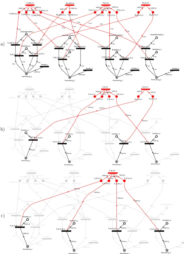
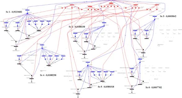
In the following chapter of this thesis, the focus is on the third method of the above mentioned ones, where the aim is to nd the structure with the most promising expected behavior. In process network synthesis (PNS), there are two major classes of decisions, one is about investments and another one about the operation. Various modes of operating units for complex structures can be investigated. If there is a failure of some operating units in the structure, the optimization remains possible. For the calculation of the expected behavior, each potential scenario has to be considered in order to evaluate possible investments. All the cost parameters of the operating units are sorted out from the basic (i.e., single stage) structure in order to get solutions for dierent scenarios. In the rst stage, all the major decisions are made, e.g., investments. In the second stage volumes of the activities are determined according to the actual situations, i.e., scenarios. Consequently, the rst stage has eect on investment costs while the second stage on the operational costs. The scenarios are weighted according to the probabilities of their occurrence. An example without details only as a general impression can be seen in Figure 1.1, the detailed description of this method is presented in the following chapter via a real-life transportation problem of bio-fuels.

The resilience of the systems is a fundamental concept for large and complex systems where long-continued reliable operation has the highest importance. Modeling and assessing the resilience of systems, which is in nature complex and large-scale, has raised remarkable interest among both practitioners and researchers in the past decade. Due to this recent popularity of the topic, several denitions and numerous approaches appeared regarding the concept of resilience and the measurement of it. In this work, the resilience is dened as the system's ability to

(11)

Figure 1.1: Maximal structure of two-stage model with 3 unreliable operating units and 6 possible scenarios

remain within a certain regime in the presence of disturbances. It determines how and to what magnitude systems will change in response to these perturbations ([49], [39], [16], [22], [35]).

The human-nature relationship gets probably the greatest attention from natural scientists these days, therefore ecosystems are of high priority among large-scale and complex systems ([95] [94]). The direct measurement of the resilience of an ecosystem and identication of its thresholds remains a key concern for managing human impacts on these ecosystems and the risk of their brake down. There are numerous approaches utilizing statistics or information theory that demonstrate some utility to identifying these thresholds or transition zones between one dynamic regime and another. In this thesis, Fisher information is used to measure the size of the dynamic regime existing between thresholds of dierent regimes. This approach has been rst developed on a simplistic predatory-prey model, and then applied to the 60-year wolf-moose population dataset from Isle Royale National Park in Michigan, USA. The developed method makes it possible to calculate where a stable system has its bounds, and what the ranges of the interacting parameters are where the system keeps its stable regime independently of the perturbations. This last point has high importance since perturbations are dicult to foresee.

This approach can be applied in its present form to larger, more complicated systems as well.

Hence, Fisher information demonstrates an early promise to directly measure the resilience of a dynamic regime.

The aim of the third chapter of this thesis is to demonstrate the above mentioned two methodologies in details by two illustrative examples, which are complex enough to highlight the advan- tages and main features of the methods but simple enough to make it easy to understand these two techniques.

3

(12)

1.2 General introduction to the supply chain optimization methods under uncertainties

There are numerous examples where optimization methodologies and decomposition techniques were applied together. An accelerated Benders' decomposition with a sampling strategy is presented in Santoso et al. (2005) to design supply chain networks with uncertain parameters [87].

Bidhandi and Yusu (2011) present an approach, where again an accelerated Benders' decomposition method is involved, it is integrated into a mixed-integer linear programming (MILP) solution phase to solve a two-stage stochastic supply chain network design model where the two stages correspond to the strategic and the tactical decisions [11]. A stochastic two-stage Branch and Fix Coordination algorithmic approach has been developed to manage supply chains by determining the production topology, plant sizing, product selection, product allocation among plants and vendor selection for raw materials [2]. The goal here was the expected prot maximization over time subtracting the investment depreciation and the operational costs. Uncertainty appears in numerous properties, the net price and demand of the product, the raw material supply cost and the production cost.

It is common to dene more than one objectives when optimizing supply chains. In the work of Sabri and Beamon (2000), the optimization objectives include cost, customer service levels, and exibility. This supply chain model is for simultaneous strategic and operational planning, where the uncertainty is in the demand [86]. Three complex objectives are dened in Azaron et al. (2008), i.e., minimization of the sum of current investment and the expected costs of processing, transportation, shortage and capacity expansion; minimization of the variaty of the total cost; and minimization of the nancial risk in other words the probability of not meeting a certain budget [6]. It is a stochastic model where the uncertainty appears in the demands, supplies, processing, transportation, shortage and capacity expansion costs. A novel method has been presented in Goh et al. (2007) applying the Moreau-Yosida regularization considering two objectives, maximal prot with minimal risk. The approach is applied to a multi-stage global supply chain network problem [38]. A little bit dierent, an integrated model has been developed in order to optimize logistics and production costs associated with the supply chain members.

The demand is uncertain and the manufacturing setting is exible. Binary decision variables select companies to form the supply chain and continuous decision variables determine volumes of the production ows. It is a robust optimization model with three objectives, minimal expected total cost, minimal cost variability due to demand uncertainty and minimal expected penalty for demand unmet at the end of the planning horizon [81]. Marufuzzaman et al. (2014) developed a two-stage stochastic programming model for designing and managing biodiesel supply chains.

The model has two objectives minimizing the cost together with the emission of the supply chain. The proposed technique is an extension of a MILP and the classical two-stage stochastic location-transportation model [69].

There are so many dierent techniques that are able to consider uncertain parameters. The most likely source of uncertainty is the stochastic demand. A two-stage, stochastic programming approach for planning multisite midterm supply chains under demand uncertainty is presented

(13)

in the works of Gupta and Maranas (2000 and 2003). Decisions about the production are made here-and-now prior to the appearance of the uncertainty; and the supply-chain decisions are in a wait-and-see mode [41] and [42]. There is another extended stochastic LP model to take demand uncertainty and cash ow into consideration for medium term [96]; and a MILP model that integrates nancial consideration with supply chain design decisions by uncertain demands [66].

The source of uncertainty can be altered for example as it is in Chen and Lee (2004) where the sales prices are uncertain [18]. It is a multi-product, multi-stage and multi-period production and distribution model to reach the maximal total prot of the whole network. The environment can be stochastic as well like in the work of Leung et al. (2006), which presents a stochastic programming approach to optimize medium-term production loading plans [64].

The sources of uncertainty also can be multiple, there are several examples in the literature.

A two-stage stochastic model has been built up to analyze the strategic planning of an oil supply chain [15]. It is a scenario-based approach with three sources of uncertainty namely, oil supply, demand of the nal product and the prices of the oil and the product. The goal here is to maximize the expected net present value. Signicant dierences appeared in the results, which demonstrates that considering uncertainties is a fundamental step in decision-making processes.

Another two-stage mixed integer stochastic approach is presented in Kim et al. (2011) where the objective is to maximize the expected prot of a biofuel supply chain by several sources of uncertainty. The rst stage decisions are about the capital investments including the size and location of the processing plants, while the ows of the biomass and product in each scenario are decided in the second stage. The model is formulated and implemented in GAMS [55]. A hybrid robust-stochastic approach is introduced in [54], where the focus is on prot maximization for closed-loop supply chain networks considering uncertainty in the transport, in the demands and returns. The solution method is based on a stochastic accelerated Benders' decomposition.

Related to supply chain networks, there are tremendous other aspects and approaches developed. For example, a MILP optimization problem has been built up to design multiproduct and multi-echelon supply chain network where the network consists of a number of manufacturing sites and a number of costumer zones at xed locations and a number of warehouses and distribution centers of unknown locations (selected from a potential location set). The objective is the minimization of the total annual cost of the network and decisions are made to determine the number, location and capacity of warehouses and distribution centers, the transportation links, as well as the ows and production rates of materials [106]. A multi-criteria genetic algorithm has been applied to a distribution problem among a number of sources and a number of destinations. The method combines analytic hierarchy processes with genetic algorithms and there is the possibility to give weights for criteria using pairwise comparison approach [17]. An- other warehouse location problem has been solved considering the variability of the demand is the only uncertain parameter [1]. A robust network design model has been developed to optimize location-allocation problem by the minimal overall cost [52]. In the work of Bertsimas and Youssef (2019), a novel robust optimization approach is detailed that is to analyze and optimize the expected performance of supply chain networks considering uncertainty in the demand ([10]).

5

(14)

Parallelly with the development of new technologies and methods, numerous simulation tools evolved in order to analyze supply chains. Petrovic (2001) details simulation tool SCSIM appli- cable to study supply chain behavior and performance if the costumer demand, external supply of raw materials and lead times to the facilities are uncertain [82]. An iterative hybrid analytic and simulation model has been developed in order to solve the integrated production-distribution problem in supply chain management, where operation time is considered as a dynamic factor in the work of Lee and Kim (2002) [63].

Understanding the contractual forms and their economic implications is a crucial part of supply chain performance evaluation. These contracts dene the independent parties coordinating the whole supply chain and answers the questions who controls what decisions and how parties would be compensated [62].

More then 85% of the world energy needs is covered by fossil-based fuels that are nite and unsustainable [12]. The importance of environmental protection and the tightness of its regularization is increasing therefore in the latest decades new alternative sources for fossil-based fuel have been widely studied [59]. One of the alternative to petroleum-based diesel fuel is the biodiesel that is considered as a renewable and natural energy source since it is made of vegetable oils and animal fats. It is a cleaner-burning diesel replacement fuel that operates in compression- ignition engines or Diesel engines and has very similar physical properties to conventional diesel fuel [24]. Besides, in the beginning of the 21st century, the traditional supply chain network of procurement, production, distribution and sales was extended to the whole lifecycle of the product by the business processes [27]. Currently, logistics and supply chain management are regarded as critical business concerns and if they are optimal, they can provide huge advantage in the competition among businesses [20]. Numerous methods and techniques in the latest decades have been developed to tackle the problem designing supply chain networks or identifying and handling the uncertainties of such systems. Researchers have viewed this issue from several aspects and have restricted the eld to many specic applications and case studies.

An accelerated stochastic Benders' decomposition technique has been developed for planning the investments of petroleum products supply chain represented by a stochastic two-stage model [79]. Another stochastic planning model for a biofuel supply chain under demand and price uncertainties is presented in Awudu and Zhang (2013) [5]. It is a stochastic LP model for maximizing the expected prot where the products' demands are uncertain but with known distribution. The applied technique comprises Benders' decomposition and Monte Carlo simulation.

For strategic planning of bioenergy supply chain systems and optimal feedstock resource allocation under supply and demand uncertainties stochastic MILP models have been applied e.g., a two-stage model developed with a Lagrange relaxation based decomposition algorithm [19].

Awudu and Zhang (2012) presented the general structure of the biofuel supply chain with three type of decisions strategic, tactical and operational [4]. The supposed sources of uncertainty are the biomass supply, transportation, production and operation, demand and prices. They studied dierent modelling techniques, like analytical and simulation methods with respect to sustainability considering environmental, economic and social aspects. Another related research is presented in Gebreslassie et al. (2012) where a multiperiod, bicreterion stochastic MILP model

(15)

has been developed to design optimal hydrocarbon biorenery supply chains where the demand and supply are uncertain [36]. A two-stage stochastic model has been built up to achieve maximal expected prot in a bioethanol supply chain under jointly appearing uncertainties, such as switchgrass yield, crop residue purchase price, bioethanol demand and sales price [80]. Shabani and Sowlati (2016) introduced a hybrid multi-stage stochastic programming robust optimization model to simultaneously include uncertainty in biomass quality and biomass availability [93].

Since the beginning of the 21st century, the importance of thinking green and therefore the signicance of green supply chains has been increasing. Mirzapour Al-e-hashem et al. (2013) have developed a stochastic programming approach for a multi-period multi-product multi-site aggregate production problem in a green supply chain where uncertainty appears in the demand.

Their model is a MILP converted into an LP by applying some theoretical and numerical techniques [75]. Another two-stage stochastic approach has been built up in order to design green supply chains considering carbon trading environment. The uncertainty lays in the product demand and the carbon price [84].

A dynamic, spatially explicit and multi-echelon MILP modelling framework is detailed in the work of Dal-Mas et al. (2011) to help assessing economic performances risk on investment of the entire biomass-based ethanol supply chain [23]. A multi-period and multi-echelon MILP model has been developed to design and plan bioethanol upstream supply chain considering that the market is uncertain. The approach has an economic value to the overall GHG emission implemented through an emissions allowances trading scheme [37]. A slightly dierent approach has been built up to dene the set of all Pareto-optimal congurations of the supply chain simultaneously taking into consideration the eciency and the risk. The latter is measured by the standard deviation of the eciency. The approach is an extended branch-and-reduce algorithm that applies optimality cuts and upper bounds to eliminate parts of the infeasible region and the non-Pareto-optimal region [51]. A similar approach is introduced in Bernstein and Federgruen (2005) where a two-echelon supply chain model is presented with a single supplier servicing a network of retailers [7]. Retailers face uncertain (random) demands and the distribution may depend only on each the retailer's own price (noncompeting) or on its own price as well as those of the other retailers (competing).

An example is presented in Tan & Aviso (2016) that is closely related to method to be presented herein [101]. It proposes an extension and generalization of the multi-period P-graph framework [48]. It suggests that the multi-period approach may be applied to robust network synthesis involving multiple scenarios instead of time periods.

1.3 General introduction to resilience in ecosystems

Internal and external drivers, like climate change, human activity, species extinction and several other causes constantly interact with dynamic ecosystems.([107], [98], [92]). The resilience of an ecosystem, as dened by the system's ability to remain within a particular regime in the presence of disturbances, determines how and to what magnitude ecosystems will change in response to these drivers ([49], [39], [16], [22], [35]). It is essential to understand the mechanisms

7

(16)

of ecological resilience to natural and anthropogenic disturbances if the vulnerability of systems to regime-changing disturbances is to be measured ([109], [67], [99], [98], [65]) and managed.

The movement of a system from one regime (or alternative stable state) to another is called regime change, and can be triggered by either exogenous disturbances (such as re or the introduction of disease), or internal causes (e.g., loss of species, increased mortality, etc.; [97]). The system's resilience to that certain disturbance determines the likelihood of regime change; in other words, its ability to maintain itself in that regime through internal feedbacks and interac- tions ([89], [29]). Note that in this work, the focus is on one regime as the measure of resilience, and not multiple regimes or the recovery of a system to a previous regime after disturbance (where recovery time is an alternative measure of resilience; see Grimm and Wissel (1997). The identication of the location of regime boundaries, also known as thresholds or tipping points, is of critical importance as early warning systems for the management and sustainability of coupled human-environment systems ([43], [90], [88], [50], [97], [99]).

Holling (1973) adopted a quantitative view of the behavior of ecological systems. Since then perspectives on ecosystem resilience have been expanded and rened to explicitly consider non- linear dynamics, boundaries, uncertainty and unpredictability, and how such dynamics interact across dierent time and spatial scales ([16], [28], [13], [88], [109], [91]). Generally, resilience may be estimated by computing the eigenvalues of the system at its equilibrium ([60]), but this approach does not provide any information about the behavior of a system close to its limits, right before the patterns decay.

Neubert and Caswell (1997) investigated several measures of a transient response, such as the biggest proportional deviation that can be generated by any perturbations, the maximal possible growth rate that directly follows the perturbation, and the time at which the amplication occurs. Scheer et al. (2015) presented methods based on the critical slowing down phenomena, which implies that recovery upon small perturbations becomes slower as a system approaches a regime threshold. In their research they also characterized the resilience of alternative regimes in probabilistic terms, measuring critical slowing down by using generic indicators related to the fundamental properties of a dynamic system ([91]). Levine et al. (2016) studied Amazon forests and reported contradictory predictions in the sensitivity and ecological resilience of them to changes in climate, sometimes resulting in biomass stability, other times in catastrophic biomass loss; transitions between regimes was continuous (no thresholds observed). Other drivers are also able to amplify climate change-driven transitions between forests and savanna globally, e.g. re disturbances, grazing, logging or other anthropogenic activities ([70]). The key to the identication of these ecosystem transitions is the availability of long-term data, which is expensive and resource-intensive.

Information Theory has been applied to assess the sustainability of dynamic systems ([85], [25]), mainly to detect transitions from one dynamic regime to another ([71]; [53], [97], [26], [100], [108]). The ball and cup mental model has been central to this work ([40]). As common analogy for dynamic regimes, the ball, representing a system that moves within a cup, representing a specic regime. The ability of the ball to remain in that same cup (or basin of attraction) means the resilience of the system ([39]). To functionally relate resilience to regimes and regime change,

(17)

two things must be determined 1) how large the cup is (regime resilience), and 2) whether the system is in the cup or outside of it (regime shift). In this work, Fisher information is applied to identify the boundaries of the regime (the size and depth of the cup) relative to the position of the ecological system (the ball) from actual values of system variables. It moves the state of the science beyond discussing symbolic cups meant to represent basins of attraction to working with the actual basin of attraction for the system, which is primary importance of this work. Unlike in prior studies (e.g., [100]), where boundaries were identied post-regime shift, it is possible to identify regime boundaries before the system has a regime change as it is demonstrated in this work. This is important because knowing the size and shape of the basin of attraction provides the opportunity to take remedial action to keep the system away from the regime boundaries before a shift has occurred. (Or, conversely in a restoration attempt, how far a system will need to be pushed in order to ip it into a more desirable regime.) The concept is illustrated with a simple modeled system and with a two-species predator-prey system (the wolves and moose population of Isle Royale National Park, Michigan USA). It is further shown that Fisher information can determine the range of predator-prey abundance over which the ecosystem remains in one regime, and hence exhibits resilience.

1.4 Introduction to Fisher Information Theory

The concept now known as Fisher information was rst introduced by the statistician Ronald Fisher (1922) regarding tting a parameter to data. Starting from the seminal work of Fisher, an expression for computing the Fisher information ([72]) from time series has been developed with the form of,

I= Z 1

p(s) dp(s)

ds ²

(1.1) where p(s) is now the simple probability density for observing particular values of s, and dp(s)/dsis the slope ofp(s).

Fisher information is also closely related to the orderliness of dynamic systems. A very ordered dynamic system is where repetitive observations of the system provide about the same result. When the system has one observable variables, this means that measuringsrepeatedly gives about the same value. In that case, p(s)is very narrow and sharp around the mean of s, and the slope dp(s)/ds is a high value. The Fisher information is proportional to [dp(s)/ds]², therefore the Fisher information has also a correspondingly high value. In the extreme case of a system where the measurable variables are constant, the system is said to be perfectly orderly, dp(s)/ds→+∞, and the Fisher information is positive innity. For a very disorderly dynamic system with again one observable variable s, each measurement of s provides a more or less dierent value. Therefore, p(s) is broad and relatively at, and the slope dp(s)/ds of p(s) is close to zero. Correspondingly, the Fisher information for a very disorderly dynamic system is near zero. In the extreme situation where a system completely lacking order, each measurement of s yields a dierent value. Then, p(s) is at, dp(s)/ds is zero, and the Fisher information

9

(18)

for this completely disorderly system is exactly zero. In summary, the Fisher information of an ordered system is high and that of a disordered system is low. One should also note the work of Al-Saar and Kim (2017) which explored the mathematical behavior of Fisher information under dierent perturbations and oscillatory regimes with possible implications for small populations of one species.

The aforementioned arguments apply also for systems that have more than one observable variable, but in such casesrepresents an n-dimensional state of the system which depends on all of the observable variables of the system. Hence, a state of the systems for a dynamic system withnmeasurable variablesx₁, x₂, . . . x_n is dened by a certain value of each of thenvariables.

Even two states that dier by the value of only one variable mean dierent states of the system.

Note that this can lead to a very large number of states of the system, each one being unique.

In order to develop a practical and calculable expression for Fisher information, consider that for a sequence of observations ofsthat have been taken over a time period, there is a one to one correlation between frequency of observations and the time over which they were taken. Hence, p(s)ds = p(t)dt where t is time, and p(t) is the probability density for sampling at a certain time. Now, T = R

dt is the total time over which the observations were made. For a cyclic system, T should generally be at least equal to one cycle, if the aim is to capture changes in system behavior. Sampling at any time point is equally probable, therefore p(t) = 1/T. Then, p(s) = (1/T)/(ds/dt) where nowds/dt is the transit speed of the system in s space. Inserting these results into Equation (1.1) the following expression results for Fisher information after some manipulations,

I= 1 T

Z (t+T) t

[R⁰⁰]²

[R⁰]⁴dt⁰ (1.2)

where R⁰ ≡ ds/dt is the speed and R⁰⁰ ≡ ^d_dt²2^s is the acceleration. For the case where s(x₁, x₂, . . . x_n)depends on n measurable variables,R⁰ and R⁰⁰ can be calculated from the Eu- clidean metric in a linear space where the coordinates are again time and the measurable variables x₁, x₂, . . . x_n. This linear space is called the system phase space. ThenR⁰can be calculated from,

R⁰ ≡ds dt =

v u u t

n

X

i=1

dxi

dt ²

(1.3) andR⁰⁰can be calculated from,

R⁰⁰≡ d dt

ds dt

= 1 R⁰

n

X

i=1

dxi

dt d²xi

dt² (1.4)

where R⁰ and R⁰⁰ are the speed and acceleration tangential to the path of the system in its phase space.

In Equations (1.2), (1.3), and (1.4) are the practical expressions that can be used to calculate Fisher information. If a dierential equation model is available as in the case of the prey-predator system used in this work, the derivativesdxi/dtandd²xi/dt²can be computed directly from the

(19)

model equations. In cases where a dierential equation model is not available, the derivatives can be approximated with nite dierence methods (see [47]). There are also many cases including this study where computing the integral in Equation (1.2) is not possible analytically, and a numerical approximation is required. For such cases the Fisher information can be approximated from,

I= 1 T

(t+T)

X

t

[R⁰⁰]²

[R⁰]⁴∆t (1.5)

11

(20)

Chapter 2

Two-stage Optimization by P-graph

In this chapter, a multi-stage optimization technique based on the P-graph Framework is described in detail, and applied to a real-life biodiesel transportation problem. The goal is to nd that structure among all the feasible ones that has the most promising expected behavior. The two major classes of decisions are about investments and about the operation. By this approach, various modes of operating units for complex structures can be investigated. The optimization procedure is still possible, even if there is a failure of some operating units in the structure.

Every potential scenario has to be regarded for the calculation of the expected behavior, so that the evaluation of possible investments can be done. All the cost parameters of the operating units are sorted out from the single stage structure so the solutions for dierent scenarios can be achieved. In the rst stage, all the major decisions are made, and then, in the second stage, volumes of the activities are determined according to the scenarios. Consequently, the rst stage has eect on investment costs while the second stage on the operational costs. The scenarios are weighted according to the probabilities of their occurrence.

The novelty of the approach is described in subsection 2.3.4 regarding the parametric cost modeling and in section 2.4 where the extended model is detailed.

2.1 Illustrative example

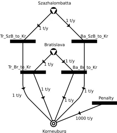
The problem, that is illustrating the approach presented hereinafter is demonstrated in this section. The task is to transport biodiesel from two locations Szazhalombatta, Hungary and Bratislava, Slovakia to a single destination Korneuburg, Austria by two dierent means of transport - barge or cargo train [Figure 2.1].

The main dierence between the two types of cargo is in their price. Barge transport is cheaper than the rail cargo, on the other hand the uncertainty is much higher in the navigability of the Danube and the availability of the docks than in the accessibility of the rail cargo. There are four possible scenarios considered regarding the above mentioned uncertainties:

• Scenario 1: All the cargo options are available

(21)

Figure 2.1: Locations of three cities in the example and the routes of the two dierent means of transport: the path of barges (blue line) and the track of rail cargo (red line) [https://www.google.hu/maps/]

13

(22)

Table 2.1: The probability of the occurrence of each scenario based on the determining factors and their probabilities

Upper

reach Lower

reach Dock in

Bratislava Dock in

SzBatta Scenario T1

Scenario T2

Scenario T3

Scenario T4

90 % 90 % 80 % 85 % Everything

is available

Barge is available only from SzB

Barge is available only from Br

Barge is not available

Y Y Y Y 0.5508

N Y Y Y 0.0612

Y N Y Y 0.0612

Y Y N Y 0.1377

Y Y Y N 0.0972

N Y N Y 0.0153

N Y Y N 0.0108

Y N N Y 0.0153

Y N Y N 0.0108

Y Y N N 0.0243

N N N Y 0.0017

N N Y N 0.0012

N Y N N 0.0027

Y N N N 0.0027

N N N N 0.0003

0.5508 0.1377 0.1692 0.1423

• Scenario 2: Barge is available only from Szazhalombatta

• Scenario 3: Barge is available only from Bratislava

• Scenario 4: Barge is not available at all

Each scenario has an estimated probability where the assessment method is considering four related factors, namely the navigability of the upper reach of the river, the navigability of the lower reach of the river and the availability of the dock in Bratislava and the dock in Szazhalom- batta. In the present instant, upper reach corresponds to the river section from Bratislava to Korneuburg and the lower reach corresponds to the river section from Szazhalombatta to Bratislava. It is also important to note, that it is assumed, if the upper reach is unnavigable, then the lower reach is unnavigable as well [Table 2.1]. The overall probability of each scenario is based on the fact that the above described four factors are independent events therefor each situation each line of the table has a certain probability value that is the product of the probability of the factors. The last line of the table presents the overall probability of each scenario, which is simply the sum of the corresponding probability values of the certain scenario.

The x and proportional costs are derived from the distance between the certain repository and the destination [Table 2.2].

(23)

Table 2.2: The x and proportional parts of the transportation costs as a function of distance

City Distance

[km] Barge x Barge

prop. [

EUR/t]

Cargo x Cargo

prop.

[EUR/t]

SzBatta

Korneuburg 300 900 9 1200 12

Bratislava

Korneuburg 100 300 3 400 4

Table 2.3: The maximal available amount of biodiesel at the source locations

Source location Maximum available ow [t/yr]

Biodiesel in Szazhalombatta 1800

Biodiesel in Bratislava 1100

There are limits for the maximal available amount of biodiesel at the source locations but each of them individually has a higher limit as the required ow at the destination, in the city of Korneuburg [Table 2.3 and 2.4]. There are also limits on the transportation capacity for all means of transportation but these upper bounds technically do not limit the transportation, since all the maximal capacities are higher than the required ow [Table 2.5].

The goal is to minimize the overall cost of this transportation problem considering the prices, limits, requirements and uncertainties as well.

In the upcoming subsection, the mathematical formulation of this illustrative example is presented; rst, the single stage problem then the extended stochastic two-stage problem.

2.1.1 Mathematical formulation of the illustrative example

In this section the mathematical formulation of the previously described illustrative example is introduced. First, the formulation of the single stage problem is presented that is the equivalent of the P-graph representation of the problem depicted in Figure 2.3. Afterwards, the mathematical formulation of the extended problem is presented that is an extension of the single stage problem into a two-stage stochastic programming problem, which is equivalent to the P-graph representation of the extended problem shown in Figure 2.4 a).

It is important to note, that all the bellow applied costs, prices and limits are the same as it is detailed in the previous section.

Table 2.4: The required amount of biodiesel at the destination

Destination Required ow [t/yr]

Biodiesel in Korneuburg 1000

15

(24)

Table 2.5: The maximal capacity of the transportation means

Means of transport Maximum capacity [t]

Barge from Bratislava 1400

Cargo from Bratislava 2000

Barge from Szazhalombatta 1600 Cargo from Szazhalombatta 2000

Decision variables of the single stage problem b_trBr the binary value of usage of train from Bratislava bbaBr the binary value of usage of barge from Bratislava b_trSzb the binary value of usage of train from Szazhalombatta bbaSzb the binary value of usage of barge from Szazhalombatta b_p the binary value of paying the penalty

xtrBr the amount of biodiesel transported by train from Bratislava x_baBr the amount of biodiesel transported by barge from Bratislava xtrSzb the amount of biodiesel transported by train from Szazhalombatta x_baSzb the amount of biodiesel transported by barge from Szazhalombatta Objective function of the single stage problem

minimize

400btrBr+ 300bbaBr+ 1200btrSzb+ 900bbaSzb+ 6666bp+ 4xtrBr+ 3xbaBr+ 12xtrSzb+ 9xbaSzb

(2.1)

subject to

x_trBr+x_baBr+x_trSzb+x_baSzb= 1000 (2.2a)

x_trBr+x_baBr ≤1100 (2.2b)

x_trSzb+x_baSzb≤1800 (2.2c)

x_trBr ≤2000 (2.2d)

x_baBr ≤1400 (2.2e)

x_trSzb≤2000 (2.2f)

x_baSzb≤1600 (2.2g)

x_trBr, x_baBr, x_trSzb, x_baSzb≥0 (2.2h) b_trBr, b_baBr, b_trSzb, b_baSzb, b_p ∈ {0,1} (2.2i)

This model is equivalent to the one described in subsection 2.3.3, where the P-graph representation is detailed and also illustrated by this example [Figure 2.3]. When uncertainty is taken

(25)

into consideration the previously dened scenarios and their probability of occurrence [Table 2.1] appear in the mathematical formulation as well. The decision variables are the same but regarding the transported amount of biodiesel there are four of each labeled with 1,2,3,4 linking them to the rst, second, third or fourth scenario respectively.

Decision variables of the extended two-stage problem b_trBr the binary value of usage of train from Bratislava bbaBr the binary value of usage of barge from Bratislava b_trSzb the binary value of usage of train from Szazhalombatta bbaSzb the binary value of usage of barge from Szazhalombatta b_p the binary value of paying the penalty

xtrBr_1,2,3,4 the amount of biodiesel transported by train from Bratislava in Scenario 1, 2, 3 and 4

xbaBr_1,2,3,4 the amount of biodiesel transported by barge from Bratislava in Scenario 1, 2, 3 and 4

xtrSzb_1,2,3,4 the amount of biodiesel transported by train from Szazhalombatta in Scenario 1, 2, 3 and 4

xbaSzb_1,2,3,4 the amount of biodiesel transported by barge from Szazhalombatta in Scenario 1, 2, 3 and 4

Objective function of the extended two-stage problem minimize

400btrBr+ 300bbaBr+ 1200btrSzb+ 900bbaSzb+ 6666bp+ + 0.5508(4xtrBr₁+ 3xbaBr₁+ 12xtrSzb₁+ 9xbaSzb₁)+

+ 0.1377(4xtrBr₂+ 3xbaBr₂+ 12xtrSzb₂+ 9xbaSzb₂)+

+ 0.1692(4xtrBr₃+ 3xbaBr₃+ 12xtrSzb₃+ 9xbaSzb₃)+

+ 0.1423(4xtrBr₄+ 3xbaBr₄+ 12xtrSzb₄+ 9xbaSzb₄)

(2.3)

17

(26)

subject to

xtrBri+xbaBri+xtrSzbi+xbaSzbi = 1000 (2.4a) xtrBri+xbaBri ≤1100 (2.4b)

xtrSzbi+xbaSzbi ≤1800 (2.4c)

xtrBri ≤2000 (2.4d)

xbaBri ≤1400 (2.4e)

xtrSzb_i ≤2000 (2.4f)

xbaSzb_i ≤1600 (2.4g)

xtrBr_i, xbaBr_i, xtrSzb_i, xbaSzb_i ≥0 (2.4h) btrBr_i, bbaBr_i, btrSzb_i, bbaSzb_i, bp_i ∈ {0,1} (2.4i) i∈ {1,2,3,4} (2.4j)

2.2 Decision tree

Decisions are made in dierent levels in those processes where uncertain parameters and factors play important role. The antecedent decisions restrict the alternatives for the later situations.

The complexity of the problem is highly aected by the number of decision levels and by the number of possible scenarios on each level [14]. There are two levels of decisions in this illustrative example, on rst level the reservation has to be dened and on second level the decision is about the utilization of the available means of transport. In Figure 2.2, the possible combinations of the rst stage decision variables are depicted with grey background (excluding penalty in order to reduce the size of the gure), while the leaves with white background represent the possibilities of second stage decision (only a some of them in order to reduce the size of the gure). Note that, penalty has to be payed if non of the transportation options satises the required demand of biodiesel at the end. In the mathematical formulation of the extended two-stage problem, the rst stage decisions are equivalent to the binary variables of each transport option and the penalty (btrBr, bbaBr, btrSzb, bbaSzb, bp), while the second stage decisions are the transported amount of biodiesel by dierent means of transport in each scenario (x_trBr_i, x_baBr_i, x_trSzb_i, x_baSzb_i and i={1,2,3,4}).

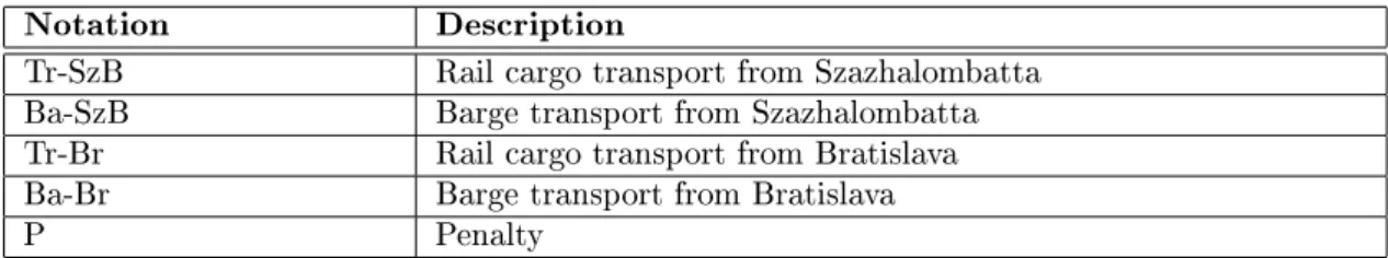
Decision trees [68] are often applied as the representation of the alternative opportunities in such problems, since these structures are comprehensible. On the other hand, decision trees easily can grow to enormous and impenetrable sizes. The simplied decision tree for the above introduced example is represented in Figure 2.2 and the regarding notations are presented in Table 2.6.

The stochastic problem has 48 825 possible alternatives, in other words there are 48 825

(27)

Table 2.6: Notation regarding the simplied decision tree

Notation Description

Tr-SzB Rail cargo transport from Szazhalombatta

Ba-SzB Barge transport from Szazhalombatta

Tr-Br Rail cargo transport from Bratislava

Ba-Br Barge transport from Bratislava

P Penalty

combinatorially dierent ways to transport biodiesel to Korneuburg applying two dierent means of transport and having two repositories and considering the 4 dierent scenarios. It also means that the decision tree has 48 825 leaves on the last stage. Certainly, by applying additional conditions the number of leaves can be reduced. By excluding the redundant transportation routes within each scenario, there are only 625 leaves remain. Even more leaves can be eliminated by excluding the unfeasible solutions. The motivational problem with the previously described parameter settings has only 240 feasible alternative solutions. Although, 240 is still too much to easily evaluate each of them.

In the following sections, a graph theoretic approach by utilizing the process graph or P-graph framework is presented that is capable of automatically generating a transparent and easy-to-use two-stage model with respect to their probability of occurrence and availability of operations in multiple scenarios.

2.3 The P-graph Framework

The P-graph methodology rooted in graph theory has been developed by Friedler, Fan and their coauthors, and initially applied for solving process-network synthesis (PNS) problems in the eld of chemical engineering process design, whose complexity is characterized by its combinatorial nature [31].

Unlike input-output models in engineering process design where operating units are represented by nodes and connected to each other through arcs, in P-graph outputs from an operating unit are not directly connected to an input to another operating unit, but instead to an another type of nodes, which are assigned to potential qualities of material streams. Arcs are leading from raw materials or from the nodes denoting qualities of input materials to the nodes representing operating units where they can be utilized and from the nodes of operating units to the nodes depicting their potential qualities of output materials or to products. P-graph unequivo- cally denes structural alternatives as material-type nodes with multiple incoming and outgoing arcs, i.e., uniquely denoting a material quality which can alternatively produced or consumed by more than one operating unit. Note that, a P-graph, where a material type node has multiple incoming or outgoing arcs, may lead to several input-output models, where outputs from and inputs to operating units that are able to produce or consume materials of the same quality are paired dierently, or mixers and splitter are incorporated in the network of operations to collect

19

(28)

20

(29)

or share the ows of materials of the same quality; see e.g. [74].

There are three cornerstones constituted by the P-graph framework, namely the graph representation of process networks, the ve axioms stating the underlying properties of the combinatorially feasible solutions, and the eective algorithms that are derived from the rst two cornerstones. The applied algorithms are for generating the maximal-structure (MSG) [32], the solution-structure generation (SSG) [31] and [30], and nally, the algorithm for determining the optimal structure (ABB) that is based on an accelerated branch-and-bound technique [33].

The P-graph framework has been applied on several elds of process synthesis since the beginning of the 1990's. These elds are optimization, and multiobjective evaluation closely related to problem introduced herein. It was implemented in the eld of business process modeling ([21], [104], [46], [105], and [102]), as well as, supply chain modeling ([56] and [61]). The P-graph framework was applied in order to solve crisis management problems ([3] and [103]), energy supply problems [110] and to minimize waste ([44] and [45] and [57]).

In the following subsections the outset, the problem denition, basic notations, and concepts are given formally as a summary of the original papers written by Friedler, Fan, and coauthors.

2.3.1 Problem Denition

A process synthesis or a process-network problem is dened by the available raw materials, potential operating units and desired products. Various properties of the operating units and materials are also given in the problem denition. These properties include the coecients for the functions expressing the costs of operating units depending on their load, and upper bounds on their respective capacities. It is often practical to specify prices and upper bounds on the availability of raw materials and similarly, lower bounds can be assessed on the desired products, which species the minimum quantity to be manufactured from the certain product by the process. In the problem specication, the relations between the materials and operating units are also included, i.e., the consumption rates of input and production rates of output materials by the operating units. The goal is to determine the optimal network where the objective can be either cost minimization or prot maximization [8].

2.3.2 Combinatorial foundation of process synthesis

There are two major steps of the mathematical programming approach to process synthesis, mathematical model generation and then solving the generated model. Both of these steps have combinatorial aspects. The rst step should express the existence or absence of links among the candidate operating units; consequently, the generated mathematical model to be solved in the second step contains integer variables. Note that the value of the objective function is often aected more drastically by the integer variables than the continuous variables in the model. Moreover, the number of integer variables, i.e., the combinatorial part of the problem aects the most the computational time. Furthermore, in practice, a process synthesis problem cannot be separated into combinatorial and continuous parts: both should be taken into account simultaneously during the solution process.

21

(30)

LetMbe a given nite nonempty set of all materials that are taken into consideration in the process synthesis. Clearly, the set of required productsPand the set of available raw materialsR are the subsets ofM. Operating units are the functional units in a process network performing various operations. Denote the set of operating units that are taken into account byO.

Throughout this chapter of the thesis, the materials are indexed by j, and the operating units, byi. Furthermore, the number of materials, i.e., the cardinality of set M, is denoted by k, while the number of operating units, i.e., the cardinality of setO, is denoted by n.

2.3.3 P-graph representation

The complexity of a process synthesis problem has an exponential relation to the number of candidate operating units, n, due to the (2ⁿ −1) possible alternative networks among which the optimal network is to be identied. Additional insights are required to eliminate redundant networks.

Each feasible process structure must conform to certain combinatorial properties. The introduction of a unique class of graphs provides the possibility to represent the structures of the process networks unambiguously and to extract these universal combinatorial properties that are inherent in all feasible processes.

Let m and o be two nite sets with

o⊆℘(m)×℘(m). (2.5)

Then, a P-graph (Process graph) is dened to be an (m,o) pair with vertex set V =m∪o and arc set A=A1∪A2 where

A1={(x, y) :y= (α, β)∈oandx∈α} (2.6) and

A2={(y, x) :y= (α, β)∈oandx∈β}. (2.7) P-graphs (Process graphs) are capable of representing process structures. For a (P,R,O) synthesis problem, let m be a subset of M, and o be a subset ofO. Furthermore, it is assumed that the sets m and o satisfy Eq.((2.5)). Therefore, the structure of the system with set m of materials and set o of operating units is formally dened as P-graph (m,o).

oi= (αi, βi) :αi, βi⊆ M (2.8) It important to note that P-graphs are directed bipartite graphs. The sets of materials and operating units are independent by denition, i.e., there are no arcs between the same vertex types. There are two disjoint sets of arcs where the elements of set A1are the arcs from materials to operating units and the elements of set A2are the arcs from operating units to materials.

The simple P-graph structure of the illustrative example is shown in [Figure 2.3]. The two

(31)

1 t/y

1 t/y 1 t/y

1 t/y

1000 t/y Bratislava

Korneuburg Szazhalombatta

Ba_Br_to_Kr Ba_SzB_to_Kr

Penalty Tr_Br_to_Kr

Tr_SzB_to_Kr

Figure 2.3: The P-graph representation of the motivational example

raw materials represent the source cities of biodiesel, the product stands for the biodiesel at the destination, and the operating units mean the two dierent cargo types from each source city to the destination and there is an additional operating unit to represent the penalty, if the fulllment does not occur. The notation used in the basic graph is the same as it was in the decision tree [see Table 2.6]. The P-graph representation of the illustrative example is equivalent to the single stage problem that is dened by mathematical formulation in the rst part of subsection 2.1.1.

2.3.4 Parametric cost modeling

The objective of the model is to minimize the overall cost of the network, which is equal to the total sum of the costs of the operating units and the prices of the raw materials.

The annual cost of an operating unit is considered as the sum of its yearly operating cost and its annualized investment cost:

annual cost=operating cost+investment cost

payout period (2.9)

The optimization model is expected to provide the optimal loads of operating units beside the optimal process structure, therefore the cost is given as function of the mass load, e.g., by a

23