A Method for Quantitative Comparison of 2D Skeletons

(1)

A Method for Quantitative Comparison of 2D Skeletons

Gábor Németh

¹

, György Kovács

²

, Attila Fazekas

³

and Kálmán Palágyi

¹

1Department of Image Processing and Computer Graphics, University of Szeged Árpád tér 2, 6720 Szeged, Hungary

{gnemeth, palagyi}@inf.u-szeged.hu

2Analytical Minds Ltd.

Árpád út 5, 4933 Beregsurány, Hungary gykovacs@analyticalminds.hu

3Department of Computer Graphics and Image Processing, University of Debrecen

Kassai u. 26, 4028 Debrecen, Hungary attila.fazekas@inf.unideb.hu

Abstract: Skeletons are widely used shape descriptors which summarize the general form of binary objects. There exist numerous skeletonization techniques that produce various skeleton-like features for the same object. Despite of the fact, that some researchers have made efforts to compare skeletons and evaluate skeletonization algorithms, we propose a new similarity measure that is based on the concept of normalized distance maps. In addition, a novel method for the quantitative comparison of skeletons is also presented. The reported method uses a high resolution dataset containing pairs of elongated objects and their expected skeletons. Our method is validated with the help of generalized morphological skeletons driven by neighborhood sequences. Based on the proposed method, we compared and ranked nineteen existing 2D thinning algorithms.

Keywords: skeleton; comparison of skeletons; generalized morphological skeleton;

neighborhood sequences

1 Introduction

Skeleton is a region-based shape descriptor which represents the general form of objects. It plays important role in various applications in image processing and pattern recognition. The skeleton of a 2D continuous object can be defined as the set of the centers of all maximal inscribed (open) disks [1]. A disk is maximal inscribed if it is included in the considered object, but it is not covered by any other inscribed disk.

(2)

Skeletonization means a process for producing an approximation to the skeleton of a discrete/digital object. There exist various skeletonization techniques that produce different skeleton-like features for the same object [2]. For example Németh and Palágyi presented 21 new algorithms in a single paper [3].

Some researchers have made efforts to compare skeletons and evaluate 2D skeletonization algorithms [4] [5] [6] [7]. They proposed some similarity measures between two skeletal sets that do not take the original elongated objects into account. The only exception is the measure of reconstructibility [5], but it may view numerous sets of points as “best” skeletons of an object. This is why we propose some new types of similarity measures that are based on normalized distance maps.

In this paper we propose a novel method, for the quantitative comparison of skeletons. The two key components of our method are a specific similarity measure for skeletons and the created gold standard image database containing 55 pairs of reference 2D images and their expected skeletons. The proposed method is validated with the help of generalized morphological skeletons driven by comparable neighborhood sequences. According to our experiments, the reported method can be used for evaluating arbitrary skeletonization algorithms.

Note that, our first attempt at this was published in a conference paper [8]. In that work the generalized morphological skeletons driven by neighborhood sequences were compared by using a small test database (containing just ten pairs of images) and we applied a similarity measure that ignore the original images.

The rest of the paper is organized as follows. Section 2 provides a method for creating a gold standard image database for comparison of skeletons. In Section 3, we propose some new similarity measures to give to the distance between two kinds of skeletons extracted from the same object. Section 4 reports the generalized morphological skeletons are combined with neighborhood sequences, furthermore we validate the proposed method with the help of generalized morphological skeletons driven by comparable neighborhood sequences. Section 5 compares 19 existing 2D thinning algorithms. Finally, we round off the paper with some concluding remarks.

2 Creation of Gold Standard Images

In this section a technique is reported for creation of gold standard images that are suitable for quantitative comparison of skeletons. It involves the following steps:

1) The selection of base images 2) The creation of reference skeletons 3) The generation of reference images These steps will now be described in more detail.

(3)

2.1 Selection of Base Images

We collected 55 high resolution binary images of different shapes. Here the selected images are called base images. Note that there are some collections of binary images (say the Kimia 216 dataset), but they contains rather small silhouettes with several thin parts. Hence all skeletonization algorithms are obliged to produce similar results for those images.

2.2 Creation of Reference Skeletons

Skeletonization algorithms need to take the following requirements into account:

 Force the “skeleton” to retain the topology of the original image (i.e., skeletonization must be a topology-preserving reduction [9])

 Force the “skeleton” to be in its geometrically correct position (i.e., in the

“center” of the object)

 Produce a minimal structure (i.e., the desired “width” of the “skeleton” is one point)

Our aim was to create the kind of reference skeletons from the base images that would meet these three conditions. In order to fulfill the first requirement, we extracted a topologically correct raw skeleton from each base image using the topology-preserving thinning algorithm AK² [10]. These raw skeletons may include some unwanted side branches. So as to satisfy the other two conditions, raw skeletons were corrected. This pruning process could be performed automatically [11], but we edited the 55 raw skeletons manually. As a result, our reference skeletons satisfy all of the three conditions listed above.

Note that method for generating reference skeletons from the base images is not significant, since any topologically correct skeletonization algorithms would do.

2.3 Generation of Reference Images

It must not be assumed that a reference skeleton is the expected skeleton of the corresponding base image. Hence we constructed reference images to replace base images.

The first step is to calculate (error free) Euclidean distance maps from the white (i.e., non-object) points of base images, where each element p has a value that gives the Euclidean distance to the nearest white point [12] [13]. The Euclidean distance map is defined as follows:

𝐷𝑀𝑤𝐵𝐼(𝑝) = min𝑞∈𝑤𝐵𝐼𝑑𝐸(𝑝, 𝑞), (1)

where wBI and 𝑑_𝐸(𝑝, 𝑞) denote the set of white points in base image BI and the Euclidean distance between points p and q, respectively. Note that DM_wBIis stored in an array of floating point numbers.

(4)

(a) (b) (c)

(d) (e) (f)

Figure 1

Creating a pair of reference skeleton and reference image. A 115×90 base image of an elephant (a); its raw skeleton (b); Euclidean distance map calculated from the white points of the base image (c);

reference skeleton (d); the reference image (here we used the raw skeleton) (e); the difference image (i.e., “base image” XOR “reference image”) (f).

The set of object points RI in the reference image is generated as follows:

𝑅𝐼 = ⋃_{𝑝∈𝑅𝑆}∆_𝐸(𝑝, 𝐷𝑀_𝑤𝐵𝐼(𝑝)) (2)

where RS is the set of skeletal points in the corresponding reference skeleton, DM_wBI is the Euclidean distance map calculated from the white points in the base image BI, and ∆_E(p,r) denotes the “best” discrete approximation to the Euclidean disk of radius r∈ℝ centred at point p∈ℤ², that is,

∆_𝐸(𝑝, 𝑟) = {𝑞 | 𝑞 ∈ ℤ², 𝑑_𝐸(𝑝, 𝑞) ≤ 𝑟} (3) In other words, the generated reference image RI is the union of disks that are centred at skeletal points in RS and the radii of these disks are determined by using the Euclidean distance map DM_wBI .

Figure 1 provides an illustrative example of creating a pair of reference skeleton and reference image. One may say that the procedure of reference skeleton construction introduces a strong bias. These reference skeletons are subjective indeed. That is why we do not consider reference skeletons as expected ones of the base images. Reference images paired with reference skeletons differ from the corresponding base images (see Figure 1f). We assumed that the reference skeleton RS is the expected discrete skeleton of the reference image RI. Note that it is not guaranteed, that for each p∈RS, disk ∆E(p,DM_wBI(p)), is a maximal inscribed one in RI, but we insist that reference skeletons satisfy all the three conditions for skeletonization methods.

All of the 55 pairs of reference images and reference skeletons, are available at https://www.inf.u-szeged.hu/~gnemeth/compskel/

(5)

3 Similarity Measures for Skeletons

3.1 Existing Similarity Measures

If we have a gold standard (i.e., reference skeleton images associated with reference images of elongated objects), then measuring the goodness of skeletons produced by an algorithm seems to be a fairly simple task. Numerous measures have been proposed to define the similarity/distance between two sets of points [4]

[5] [6].

Let us consider the frequently applied Hausdorff distance between two (arbitrary) sets of points P and Q, which may be defined as follows [14]:

𝐻(𝑃, 𝑄) = max{ max_𝑝∈𝑃min_𝑞∈𝑄𝑑_𝐸(𝑝, 𝑞), max_𝑞∈𝑄min_𝑝∈𝑃𝑑_𝐸(𝑝, 𝑞) }, =

max { max𝑝∈𝑃𝐷𝑀𝑄(𝑝) , max𝑞∈𝑄𝐷𝑀𝑃(𝑞) } (4) where DM_P(q) denotes the value of the Euclidean distance map calculated from the set of points P at position q.

In our first attempt, we sought to make a comparison of the skeleton S (extracted from a reference image) with the corresponding reference skeleton RS using the similarity measure H(S,RS), but it did not work. Just one salient point (like an endpoint of an unwanted line segment) in S may determine H(S,RS), hence it is not a fair assessment of a method.

Lee, Lam, and Suen [5] proposed a sophisticated similarity measure between two skeletons P and Q which is defined by the following Formula (5):

𝐶(𝑃, 𝑄) = (_#(𝑃)¹ ∑ _𝐷𝑀 ¹

𝑄(𝑝)²+1

𝑝∈𝑃 +_#(𝑄)¹ ∑ _𝐷𝑀 ¹

𝑃(𝑞)²+1

𝑞∈𝑄 ) / 2 (5)

where #(P) denotes the number of points in set P.

Similarly to the Hausdorff distance and others proposed in some studies [4] [5]

[6], measure C does not take into account the original (elongated) object. Hence we do not regard these similarity measures as acceptable for evaluating skeletons.

Skeletons should be treated as special kinds of sets of points.

Lee, Lam, and Suen [5] proposed an additional measure that takes the original object into account. This measure of reconstructibility is defined by the formula

𝛼(𝑆, 𝐼) =^#(⋃^𝑝∈𝑆^∆^𝐸_#(𝐼)^{(𝑝,𝐷𝑀}^𝑤𝐼^(𝑝))⁾ (6)

where S is a “skeleton” of object I. The measure takes values from the interval [0,1], since ⋃_𝑝∈𝑆∆𝐸(𝑝, 𝐷𝑀𝑤𝐼(𝑝))⊆ 𝐼. They say that: α(S,I)=1 means that S is identical to the “best” skeleton of image I. Unfortunately, this is not always the case. There is no guarantee that an Euclidean disk included in I and centred at 𝑝 ∈ 𝑆 with radius ∆𝐸(𝑝, 𝐷𝑀𝑤𝐼(𝑝)) will be a maximal inscribed one. One can construct various sets of point S⊆I such that ⋃𝑝∈𝑆∆𝐸(𝑝, 𝐷𝑀𝑤𝐼(𝑝))= 𝐼. In

(6)

addition, it is not hard to see that α(I,I)=1 (for any object I), but an elongated object may not be treated as the “best” skeleton of itself.

Note that Couprie and Bertrand [15] also proposed some measures (i.e., spuriousness factor, reconstruction error, thickness factor) between 3D curve- skeletons, however these measures can be calculated in a complex way furthermore do not consider the thickness of different parts of objects. In addition, their approach does not yield a fully automated method.

Sobieczki et. al. [16] [17] also investigated some similarity measures to compare 3D mesh-contraction-based curve-skeletonization algorithms. Unfortunately, they assumed mesh representation, hence their method cannot be applied for pixel- based images.

Some shape matching algorithms are based on skeletal graphs. Skeletal graphs are derived from 3D curve-skeletons or 2D centerlines in which endpoints and junction points represents the set of nodes/vertices, and there is an edge between two nodes if the corresponding pixels/voxels are connected by a skeletal path.

These methods consider pruned skeletons (i.e., some unwanted branches are removed [11]), and they are based on some time consuming graph matching methods [18] [19] [20] [21] [22]. Unfortunately, the similarity measures that are used in graph matching methods are not skeleton-specific ones, they assume general sets of points, and do not take the original object into consideration.

Note that chamfer matching [23] [24] could also yield a similarity measure, where the query and the target contours are the two skeletons to be compared.

Unfortunately, the original object would be also ignored, and chamfer distances are to approximate the Euclidean metric with integers (or rational numbers).

Despite the wealth of previously proposed similarity measures, we looked for new ones. It should be mentioned that in our previous paper [8], we applied five kinds of similarity measures which also ignored the original objects.

3.2 Distance Map Normalization

From the results of our experiments, we came to realize that not every skeletal point is equally important (i.e., positioning error of a certain size in a “thin” part is much more serious than the same error in a “thick” segment). This is why we propose a normalized distance map which is defined as:

𝐷𝑀𝑆,𝑤𝐼= 𝐷𝑀𝑆/(𝐷𝑀𝑆+ 𝐷𝑀𝑤𝐼) (7)

where S is a set of skeletal points that is extracted from the image I by a skeletonization algorithm. (Note that “/” and “+” merely denote the point-by-point division and addition of two arrays of floating point numbers which have the same size, respectively.) Figure (2) shows normalized distance maps for five kinds of skeletons (see Section 4).

(7)

RI 𝐷𝑀_{𝑅𝑆,𝑤𝑅𝐼} 𝐷𝑀𝑆𝑆(𝑅𝐼,<1>),𝑤𝑅𝐼

𝐷𝑀𝑆𝑆(𝑅𝐼,<2>),𝑤𝑅𝐼 𝐷𝑀𝑆𝑆(𝑅𝐼,<1,2>),𝑤𝑅𝐼 𝐷𝑀_{𝑆𝑆(𝑅𝐼,𝒜}_𝑜𝑝𝑡_{),𝑤𝑅𝐼}

Figure 2

A reference image RI (see Fig. 1e); the corresponding normalized distance maps of its reference skeleton RS (see Fig. 1d) and the four kinds of skeletons shown in Fig. 5

It can readily be seen that the following three properties hold:

 0 ≤ 𝐷𝑀𝑆,𝑤𝐼(𝑝) ≤ 1 for each point p∈wI

 𝐷𝑀𝑆,𝑤𝐼(𝑝) = 0 if and only if p∈S

 𝐷𝑀𝑆,𝑤𝐼(𝑝) = 1 if and only if p∈wI

3.3 A New Similarity Measure Based on Normalized Distance Maps

Let us consider the following measure between a skeleton S of image I and a normalized distance map 𝐷𝑀_{𝑆,𝑤𝐼}:

𝐷𝑎𝑣𝑔(𝑆, 𝐷𝑀𝑆,𝑤𝐼) =_#(𝑆)¹ ∑𝑝∈𝑆𝐷𝑀𝑆,𝑤𝐼(𝑝) (8) We are now ready to introduce a new similarity measure that is recommended for comparing two skeletons:

𝐴𝐴𝐼(𝑆₁, 𝑆2) = (𝐷_𝑎𝑣𝑔(𝑆1, 𝐷𝑀𝑆₂,𝑤𝐼) + 𝐷𝑎𝑣𝑔(𝑆2, 𝐷𝑀𝑆₁,𝑤𝐼)) /2 (9) where S1 and S2 are two skeletal sets of points that are extracted from the same image I (S₁,S₂⊆I). In addition the following three properties hold for the similarity measure AA (for any S1, S2, and I):

 0 ≤ 𝐴𝐴𝐼(𝑆1, 𝑆2) ≤ 1

 𝐴𝐴_𝐼(𝑆₁, 𝑆₂) = 𝐴𝐴_𝐼(𝑆₂, 𝑆₁)

 𝐴𝐴𝐼(𝑆₁, 𝑆1) = 0

(8)

We should stress here, that the smaller value means a better similarity between the two skeletons in question.

3.4 Goodness of Similarity Measures

Consider two skeletonization techniques T1 and T2 that produce skeletal sets of points T₁(I) and T₂(I) for image I. Suppose that it is known that T₁ is better than T₂ (i.e., T₁ can produce more reliable skeletons than T₂). Let (RI,RS) be a pair of reference image and its reference skeleton.

We say that the similarity measure SM is reasonable for (RI,RS) if

𝑆𝑀_𝑅𝐼(𝑇₁(𝑅𝐼), 𝑅𝑆) ≤ 𝑆𝑀_𝑅𝐼(𝑇₂(𝑅𝐼), 𝑅𝑆) (10) The purpose of our experiments was to show that the proposed similarity measures is reasonable. The question is: How to find such comparable skeletonization techniques T₁ and T₂?

4 Validation

4.1 Comparable Skeletons

In this section a new family of skeletons called sequence skeletons are introduced.

These skeletons are not competitive with others produced by some existing skeletonization algorithms but we can validate our comparison method with the help of them.

Mathematical morphology, developed by Matheron and Serra [25], is a powerful tool for image processing and image analysis. Its operators can extract relevant topological and geometrical information from images by using structuring elements (i.e., geometric templates to probe some properties of interest) of various shapes and sizes. We use the fundamental concepts and notions of mathematical morphology as reviewed by Gonzalez and Woods [26].

4.1.1 Neighborhood Sequences and their Disks

The aim of this subsection is twofold. First, notions and results related to neighborhood sequences and the derived discrete distances will be reviewed in brief. Second, the disks corresponding to the neighborhood sequences will be formally expressed in terms of dilations (i.e., fundamental morphological operations) [26].

We will now present some basic notions and results concerning neighborhood sequences.

(9)

Let n,m ∈ ℕ with m ≤ n. Two points p=(p1, …, p_n) and q=(q₁, …, q_n) in ℤⁿ are said to be m-adjacent if both of the following conditions are satisfied:

 |𝑝_𝑖− 𝑞_𝑖| ≤ 1 (𝑖 ∈ {1,2, … , 𝑛})

 ∑^𝑛_𝑖=1|𝑝_𝑖− 𝑞𝑖| ≤ 𝑚

Note that these relations are reflexive and symmetric. In the case of n=2 (i.e., the 2-dimensional orthogonal grid), 1– and 2–adjacency relations are often referred to as 4– and 8–adjacencies, respectively [9].

The sequence 𝒜=<A(1),A(2),…> is called an nD–neighborhood sequence if A(i)∈{1, 2, …, n} for all i∈ℕ. If for some t∈ℕ, we have A(i+t)=A(i) for all i∈ℕ, then the neighborhood sequence 𝒜 is called periodic with period t. For simplicity, let 𝒜=<A(1),…,A(t)> stand for a periodic neighborhood sequence having a period t.

Let 𝒜=<A(1),A(2), …> be an nD–neighborhood sequence. The sequence of points <r₀,…, r_l> (r_j∈ℤⁿ, j∈{0,…, l}) is an 𝒜-path of length l (l ≥ 0) from point p to point q if p=r₀, q=r_l, and r_j−1 and r_j are A(j)-adjacent for all j (j∈{1, …, l}).

Let d𝒜 (p, q) stand for the 𝒜-distance between two points p and q. It is defined as the length of the shortest 𝒜-path(s) between p and q.

As we are considering 2D binary images, we shall now examine 2D neighborhood sequences. According to the definitions above, 2D–neighborhood sequences may contain two kinds of elements, namely “1” and “2”. Notice that distances d_<1>, d_<2>, and d<1,2> correspond to cityblock, chessboard, and octagonal distances, respectively [27]. It can readily be seen that there exist an infinite number of possible neighborhood sequences. The trick is to choose the neighborhood sequence which gives the best approximation to the Euclidean distance. The existence of the best approximating neighborhood sequence was proved in [28].

This non-periodic sequence is:

𝒜𝑜𝑝𝑡= < 2,1,1,1,2,1,2,1,1,2,1,1, . . . > (11) Let d_E(p, q) represent the Euclidean distance between the two points p and q in ℤ². A natural partial ordering relation “≼” can be defined for 2D–neighborhood sequences 𝒜1 and 𝒜2.

If |d𝒜1(p, q) − d_E(p, q)| ≤ |d𝒜2(p, q) − d_E(p, q)| (for any two points p and q), then 𝒜1 ≼ 𝒜2 (i.e., 𝒜1 is better than 𝒜2).

The following conditions hold for the four neighborhood sequences under comparison [28]:

𝒜𝑜𝑝𝑡≼ < 1,2 > ≼ < 1 >

𝒜𝑜𝑝𝑡≼ < 1,2 > ≼ < 2 > (12)

(10)

4 4 3 4 4 3 2 3 4 4 3 2 1 2 3 4 4 3 2 1 0 1 2 3 4

4 3 2 1 2 3 4 4 3 2 3 4

4 3 4 4

∆<1>

4 4 4 4 4 4 4 4 4 4 3 3 3 3 3 3 3 4 4 3 2 2 2 2 2 3 4 4 3 2 1 1 1 2 3 4 4 3 2 1 0 1 2 3 4 4 3 2 1 1 1 2 3 4 4 3 2 2 2 2 2 3 4 4 3 3 3 3 3 3 3 4 4 4 4 4 4 4 4 4 4

∆<2>

4 4 4 4 4 4 4 3 3 3 4 4 4 4 3 2 2 2 3 4 4 4 3 2 2 1 2 2 3 4 4 3 2 1 0 1 2 3 4 4 3 2 2 1 2 2 3 4 4 4 3 2 2 2 3 4 4

4 4 3 3 3 4 4 4 4 4 4 4

∆<1,2>

Figure 3

Sample disks corresponding to the cityblock, chessboard, and octagonal distances of radii up to 4. The points denoted by a “0” are the origin and each point denoted by r≤k belongs to a disk of radius k.

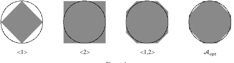
<1> <2> <1,2> 𝒜_𝑜𝑝𝑡

Figure 4

Approximations of the Euclidean disk of radius 96 (represented as a black circles) considering four neighborhood sequences <1>, <2>, <1,2>, and 𝒜_𝑜𝑝𝑡.

𝒜𝑜𝑝𝑡≼ < 1,2 > ≼ < 1 >

𝒜_𝑜𝑝𝑡≼ < 1,2 > ≼ < 2 >Let us consider the discrete distance d𝒜 based on the neighborhood sequence 𝒜. The corresponding discrete disk of radius k (k=0,1, …) centred at the origin 𝒪 is defined by

∆_𝒜(𝑝) = { 𝑝 | 𝑑_𝒜(𝒪, 𝑝) ≤ 𝑘 } (13)

Figure 3 shows some discrete disks derived from the three periodic discrete distances d_<1>, d_<2>, and d<1,2>.

It is well known that the neighborhood sequences <1> and <2> (which are composed of only one kind of adjacency relation) are diamond–shaped and square–shaped, respectively, and we can get various octagon–shaped discrete disks if both relations are combined.

In order to get discrete disks based on neighborhood sequences in terms of dilations, we will assign structuring elements to adjacency relations.

Let us consider the m-adjacency in ℤ² (m=1,2). The structuring element Y(m) for the m-adjacency is defined by:

𝑌(𝑝) = { 𝑝 | 𝑝 ∈ ℤ² such that 𝑝 is 𝑚-adjacent to 𝒪 } (14) Since m-adjacency is a reflexive and symmetric relation over ℤ², the structuring element Y(m) contains the origin and it is symmetric, i.e., if p=(p1,p2)∈Y(m), then

−p=(−p1,−p2)∈Y(m).

(11)

It can readily be seen that the discrete disk ∆𝒜(k) can be expressed in terms of dilations (denoted by “⊕” [26]) as follows

∆𝒜(𝑘) = {{𝒪} if 𝑘 = 0

∆_𝐸(𝑘 − 1)⨁𝑌(𝐴(𝑘)) otherwise

= (… ({𝒪}⨁𝑌(𝐴(1))) ⨁ …) ⨁𝑌(𝐴(𝑘)) (15) Approximations of Euclidean disks with the structuring elements (or discrete disks) derived from four kinds of neighborhood sequences are illustrated in Figure 4.

4.1.2 Generalized Morphological Skeletons Driven by Neighborhood Sequences

The skeleton of a discrete binary image can be characterized via morphological operations. In this section first the conventional morphological skeleton that just uses one structuring element will be reviewed. Then we will focus on the generalized morphological skeletons that are driven by neighborhood sequences.

The 2D morphological skeleton S(X,Y) of a discrete set of points X⊂ℤ² (i.e., object points in a 2D binary image) determined by a structuring element Y consists of the centers of all maximal inscribed discrete disks of radius k (k=0,1,...) [26]. With this approach, the structuring element Y is assumed to be the unit disk (i.e., a disk of radius 1) and the discrete disk Y^k of radius k is derived from Y by successive dilations:

𝑌^𝑘 = {{𝒪} if 𝑘 = 0, 𝑌^𝑘−1⨁𝑌 otherwise = (… (({𝒪}⨁𝑌)⨁𝑌) ⨁ …)⨁𝑌⏟

𝑘−times

(16) A point p∈X is the center of a maximal inscribed discrete disk of radius k (k =0,1,…) if p∈X⊖Y^k and p∉(X⊖Y^k+1)⊕Y , where “⊖” denotes the erosion (i.e., a fundamental morphological operation that is dual to dilation) [26].

For this reason, the morphological skeleton MS of a set X determined by a structuring element Y is defined by:

𝑀𝑆(𝑋, 𝑌) = ⋃^𝐾_𝑘=0𝑀𝑆_𝑘(𝑋, 𝑌)

= ⋃^𝐾_𝑘=0(𝑋 ⊖ 𝑌^𝑘) − [(𝑋 ⊝ 𝑌^𝑘+1) ⊕ 𝑌] (17) where K is the radius of the largest inscribed disk. In other words,

𝐾 = max { 𝑘 | 𝑋 ⊖ 𝑌^𝑘≠ ∅ } (18)

According to the formulation defined by (17) and (18), the morphological skeleton is the union of the disjoint skeletal subsets, where MSk(X, Y) contains the centers of all maximal inscribed disks of radius k (k=0,1, ..., K). An interesting property of

(12)

the morphological skeleton is that, a set X, can be exactly reconstructed from the K+1 skeletal subsets:

𝑋 = ⋃^𝐾_𝑘=0𝑀𝑆_𝑘(𝑋, 𝑌) ⊕ 𝑌^𝑘 (19)

The main limitation of a morphological skeleton is that its construction is based on

“disks” of the form Y^k. If the chosen structuring element Y=Y(m) (m=1,2) (see (14)), then the discrete disk Y^k=∆<m>(k) (see (15)). Discrete disks Y^k=∆<1>(k) and

Y^k=∆_<2>(k) do not give “good” approximations to the Euclidean disks (see Figure

4), hence we suspect that morphological skeletons are probably not “close” to the expected skeleton.

In order to reduce the shortcomings of the conventional morphological skeleton, Maragos proposed generalized morphological skeleton transforms that allows us to use varying structuring elements in different steps [29]. In his approach, the structuring element Y^k (i.e., a discrete disk of radius k, see (16)) can be replaced by {O}⊕Y1⊕. . .⊕Yk, where <Y₁, …, Yk> is the prefix of length k of an arbitrary sequence structuring elements (k = 0, 1, …).

These generalized morphological skeletons can be combined with neighborhood sequences by using the sequence of structuring elements

< 𝑌(𝐴(1)), 𝑌(𝐴(2)), … > which are related to the neighborhood sequence 𝒜 =< 𝐴(1), 𝐴(2), … >.

This sequence skeleton makes use of discrete disks ∆𝒜(k) (k = 0, 1, …) (see (15)).

The sequence skeleton SS of a X⊆ℤ² driven by a neighborhood sequence 𝒜 is defined by

𝑆𝑆(𝑋, 𝒜) = ⋃^𝐾_𝑘=0𝑆𝑆_𝑘(𝑋, 𝒜) (20)

where

𝑆𝑆𝑘(𝑋, 𝒜) = (𝑋 ⊝ Δ_𝒜(𝑘)) − [(𝑋 ⊖ Δ_𝒜(𝑘 + 1)) ⊕ 𝑌(𝐴(𝑘 + 1))] (21) and K is the radius of the largest inscribed disk; that is

𝐾 = max { 𝑘 | 𝑋 ⊝ Δ𝒜(𝑘) ≠ ∅ } (22)

With this formulation defined by (20) and (22), the sequence skeleton is the union of disjoint skeletal subsets, where 𝑆𝑆𝑘(𝑋, 𝒜) contains the centers of all maximal inscribed disks ∆𝒜(k) (k=0, 1, . . . ,K).

It is easy to see that in the 𝒜=<m> case (m=1,2)

𝑆𝑆(𝑋, 𝒜) = 𝑀𝑆(𝑋, 𝑌(𝑚)) (23)

thus the conventional morphological skeleton is a special case of sequence skeletons. Some illustrative examples of sequence skeletons are given in Fig. 5.

(13)

X 𝑆𝑆(𝑋, < 1 >) = 𝑀𝑆(𝑋, 𝑌(1)) 𝑆𝑆(𝑋, < 2 >) = 𝑀𝑆(𝑋, 𝑌(2))

𝑆𝑆(𝑋, < 1,2 >) 𝑆𝑆(𝑋, 𝒜_opt) Figure 5

A 115 × 90 image of an elephant and its sequence skeletons driven by four kinds of neighborhood sequences. Notice that the first two sequence skeletons are also conventional morphological skeletons.

The reconstruction formula from the sequence skeleton SS(X,𝒜) is analogous to (19), hence:

𝑋 = ⋃^𝐾_𝑘=0𝑆𝑆_𝑘(𝑋, 𝒜) ⊕ ∆_𝒜(𝑘) . (24)

This means that like the conventional morphological skeletal subsets, the subsets of the sequence skeleton also fully represent the original set of points [29] [30].

Next, note that the connectivity of the conventional morphological skeletons and sequence skeleton is not guaranteed (i.e., these skeletons are not connected and topologically correct for numerous connected objects).

It is known that the non–periodic neighborhood sequence 𝒜opt (see (11)) provides the best approximation to the Euclidean distance and the Euclidean disk [28].

Hence we can assume that SS(X, 𝒜opt) is the best sequence skeleton for any X (i.e., it gives the best approximation to the expected skeleton).

4.2 Validation with Sequence Skeletons

In this section we validate the proposed method for the quantitative comparison of skeletons with the help of neighborhood sequences.

We examined our gold standard image database, containing 55 pairs of reference images and reference skeletons, the four suggested similarity measure AA, and the four metrical neighborhood sequences <1>, <2>, <1, 2>, and 𝒜opt (see (11)).

For each pair of (RI, RS) we calculated the followings:

 The four sequence skeletons driven by the four neighborhood sequences in question:

S1 = SS(RI, <1>)

(14)

S2 = SS(RI, <2>) S3 = SS(RI, <1, 2>) S4 = SS(RI, 𝒜opt) (see (20))

 The five normalized distance maps corresponding to the reference skeleton and the four sequence skeletons:

𝐷𝑀̅̅̅̅̅_{𝑅𝑆,𝑤𝑅𝐼} 𝐷𝑀̅̅̅̅̅_𝑆₁_{,𝑤𝑅𝐼} 𝐷𝑀̅̅̅̅̅_𝑆

2,𝑤𝑅𝐼

𝐷𝑀̅̅̅̅̅_𝑆

3,𝑤𝑅𝐼

𝐷𝑀̅̅̅̅̅_𝑆

4,𝑤𝑅𝐼 (see (7) and Fig. 2)

 The four values of similarity measures:

AA_RI(S₁,RS) AA_RI(S₂,RS) AARI(S3,RS) A_RI(S₄,RS) (see (9))

All the measures for the 55 pairs of reference images and reference skeletons, are presented in the following website:

https://www.inf.u-szeged.hu/~gnemeth/compskel/

Observe that a smaller value in a row, means a better similarity of the sequence skeleton and the reference skeleton.

We know that 𝒜opt≼<1, 2>≼<1>,<2> (see (12)), hence the following inequalities:

𝑆𝑀_𝑅𝐼(𝑆𝑆(𝑅𝐼, 𝒜_𝑜𝑝𝑡), 𝑅𝑆) ≤ 𝑆𝑀𝑅𝐼(𝑆𝑆(𝑅𝐼, < 1,2 >), 𝑅𝑆) ≤ 𝑆𝑀_𝑅𝐼(𝑆𝑆(𝑅𝐼, < 1 >), 𝑅𝑆)

should hold for a reasonable similarity measure SM, for each pair of reference image and reference skeleton (RI,RS) (see (10)). We should add that the similarity measure AA satisfies it for high resolution images (in the case of Kimia dataset the image resolution is too low to measure big differences), hence, it is judged a reasonable similarity measure. Note, as well, that none of the five types of similarity measures applied in our previous paper [8] are reasonable.

5 Results

In this section we compare and rank nineteen thinning algorithms. The similarity measure AA has been computed for the 4×55=220 morphological skeletons driven by the four neighborhood sequences <1>, <2>, <1,2> and 𝒜𝑜𝑝𝑡. In each case, 𝒜_𝑜𝑝𝑡 provided the best result.

Evaluation is based on three different ranking methods:

(15)

1) Sum of ranks: For each test image, the similarity measure AA has been calculated and the algorithms have been sorted according the AA value.

The scores have been summarized for each algorithm. The winner has the lower score value. Table 1 summarizes the result according to this ranking method.

2) Sum of AA values: The score of an algorithm has been computed as the sum of AA values for each test image. The winner algorithm has the lowest score. Table 2 shows the result according to this ranking.

3) Tournament: In a competition two algorithms play matches for each test image. If an algorithm is better (i.e., has a lower AA value) for more images than the other one in a competition, then it wins 1 point. In the tournament, the algorithms plays competitions pairwise. The best algorithm wins the most competitions. Table 3 presents the result of this ranking.

According to the our quantitative and fully automated comparison with the three types of rankings, we can state, that the 2*2-subiteration parallel thinning algorithm SI-<NE,SW,NW,SE>-E3, proposed by Németh Kardos and Palágyi [31], is the best choice, among the nineteen thinning algorithms compared.

Conclusions

A novel method for quantitative comparison of skeletons was presented herein.

The proposed method is based on a new similarity measure and a gold standard 2D image database, containing pairs of reference images with elongated objects and their expected skeletons. Our method is validated using generalized morphological skeletons, driven by neighborhood sequences. According to the experiments, the proposed method can be used for evaluating arbitrary 2D skeletonization algorithms. Based on our method, the quantitative comparison of nineteen 2D thinning algorithms were presented, as well. In future work, we plan to extend our method to evaluate 3D skeletonization techniques.

Table 1

“Sum of ranks” method

Rank Algorithm Ref. Type Sum of ranks

for each image

1 SI-<NE,SW,NW,SE>-E3 [31] sub iteration-based 535

3 BM99 [32] fully parallel 916

4 H89 [33] fully parallel 1235

6 GH92C [34] fully parallel 1344

7 GH89A1 [35] sub iteration-based 1656

8 FP-E3 [31] fully parallel 1685

10 PAV81 [36] [37] fully parallel 1862

11 EM93 [38] fully parallel 1965

(16)

13 AK² [10] fully parallel 2131

14 SI-<N,E,S,W>-E2 [31] sub iteration-based 2965

16 ZSLW [39] sub iteration-based 3146

18 RUT66 [40] fully parallel 4267

19 CWSI87 [41] fully parallel 4759

Table 2

Sum of AA values” methods

Ran k

Algorithm Ref. Type Sum of AA values

1 SI-<NE,SW,NW,SE>-E3 [31] sub iteration-based 3.3108 2 SI-<NE,SW,NW,SE>-E2 [31] sub iteration-based 3.3122 3 SI-<NE,SW,NW,SE>-E1 [31] sub iteration-based 3.7920

4 BM99 [32] fully parallel 3.8911

5 H89 [33] fully parallel 4.0083

6 PAV81 [36] [37] fully parallel 4.0200

7 GH92C [34] fully parallel 4.0210

8 FP-E3 [31] fully parallel 4.0587

10 EM93 [38] fully parallel 4.0604

11 AK² [10] fully parallel 4.1016

12 GH89A1 [35] sub iteration-based 4.1181

14 SI-<N,E,S,W>-E3 [31] sub iteration-based 5.1786

SI-<N,E,S,W>-E2 [31] sub iteration-based 5.1786

16 ZSLW [39] sub iteration-based 5.3166

17 SI-<N,E,S,W>-E1 [31] sub iteration-based 5.7857

18 RUT66 [40] fully parallel 6.9958

19 CWSI87 [41] fully parallel 9.0067

Table 3

“Tournament” methods

Rank Algorithm Ref. Type Number of winner

single combats

4 BM99 [32] fully parallel 15

5 H89 [33] fully parallel 14

6 GH92C [34] fully parallel 13

7 GH89A1 [35] sub iteration-based 12

11 PAV81 [36] [37] fully parallel 8

12 EM93 [38] fully parallel 7

(17)

13 AK² [10] fully parallel 6

14 SI4-<N,E,S,W>-E3 [31] sub iteration-based 4

SI4-<N,E,S,W>-E2 [31] sub iteration-based 4

16 ZSLW [39] sub iteration-based 3

18 RUT66 [40] fully parallel 1

19 CWSI87 [41] fully parallel 0

References

[1] P. Giblin and B. B. Kimia: A formal classification of 3d medial axis points and their local geometry, IEEE Transactions on Pattern Analysis and Machine Intelligence, vol. 26, 2004, pp. 238-251.

[2] K. Siddiqi and S. Pizer, Medial representations – Mathematics, algorithms and applications, vol. 37, Springer, 2008.

[3] G. Németh and K. Palágyi: Topology preserving parallel thinning algorithms, International Journal of Imaging Systems and Technology, vol. 21, 2011, pp.

37-44.

[4] L. Lam and C. Y. Suen: Automatic comparison of skeletons by shape matching methods, Int. Journal on Pattern Recognition and Artificial Intelligence, vol. 7, 1993, pp. 1271-1286.

[5] W. Lee, L. Lam and C. Y. Suen: A systematic evaluation of skeletonization algorithms, Int. Journal on Pattern Recognition and Artificial Intelligence, vol. 7, 1993, pp. 1203-1225.

[6] R. Plamondon, C. Y. Suen, M. Bourdeau and C. Barriére: Methodologies for evaluating thinning algorithms for character recognition, Int. Journal on Pattern Recognition and Artificial Intellelligence, vol. 7, 1993, pp. 1247- 1270.

[7] W.-P. Choi, K.-M. Lam and W.-C. Siu: Extraction of the Euclidean skeleton based on a connectivity, Pattern Recognition, vol. 36, 2003, pp. 721-729.

[8] A. Fazekas, K. Palágyi, G. Kovács and G. Németh: Skeletonization Based on Metrical Neighborhood Sequences, Proceedings of the 6th Int. Conf.

Computer Vision Systems), LNCS, vol. 5008, A. Gasteratos, M. Vincze and J.

K. Tsotsos, (eds.), Springer, 2008, pp. 333-342.

(18)

[9] T. Y. Kong and A. Rosenfeld: Digital topology: Introduction and survey,"

Computer Vision, Graphics, and Image Processing, vol. 48, 1989, pp. 357- 393.

[10] G. Bertrand and M. Couprie: New 2D parallel thinning algorithms based on critical kernels, Proceedings of the 11th Int. Workshop Combinatorial Image Analysis, LNCS, vol. 4040, R. Reulke, U. Eckhardt, B. Flach, U. Knauer and K. Polthier (eds.), Springer, 2006, pp. 45-59.

[11] D. Shaken and A. Bruckstein: Pruning Medial Axes, Computer Vision and Image Understanding, vol. 69, no. 2, 1998, pp. 156-169.

[12] G. Borgefors: Distance transformations in arbitrary dimensions, Computer Vision, Graphics, and Image Processing, vol. 27, 1984, pp. 321-345.

[13] R. Fabbri, L. F. Costa, J. C. Torelli and O. M. Bruno: 2D Euclidean distance transform algorithms: A comparative survey, ACM Computing Surveys, vol.

40, no. 2, 2008, pp. 1-44.

[14] R. Klette és A. Rosenfeld: Digital Geometry – Geometric Methods for Digital Picture Analysis, Morgan Kaufmann Publisher, 2004.

[15] M. Couprie and G. Bertrand: Asymmetric parallel 3D thinning scheme and algorithms based on isthmuses, Pattern Recognition Letters, vol. 76, 2016, pp. 21-31.

[16] A. Sobieczki, H. Yassan, A. Jalba and A. Telea: Qualitative comparison of contraction-based curve skeletonization methods, Proceedings of 11th International Symposium on Mathematical Morphology, Springer-Verlag, 2013, pp. 425-439.

[17] A. Sobieczki, A. Jalba and A. Telea: Comparison of curve and surface skeletonization methods for voxel shapes, Pattern Recognition Letters, vol.

47, 2014, pp. 147-156.

[18] C. Aslan, A. Erdem, E. Erdem and S. Tari: Disconnected skeleton: Shape at its absolute scale, IEEE Trans. Pattern Analysis and Machine Intelligence, vol. 30, no. 12, 2008, pp. 2188-2203.

[19] X. Bai and L. J. Latecki: Path similarity skeleton graph matching, IEEE Trans. Pattern Analysis and Machine Intelligence, vol. 30, 2008, pp. 1282- 1292.

[20] J. Tschirren, G. McLennan, K. Palágyi, E. A. Hoffman and M. Sonka:

Matching and anatomical labeling of human airway tree, IEEE Trans.

Medical Imaging, vol. 24, 2005, pp. 1540-1547.

[21] A. Brenneke és T. Isenberg: 3D shape matching using skeleton graphs,

(19)

Proceedings of Simulation and Visualisation, 2004, pp. 299-310.

[22] H. Sundar, D. Silver, N. Gagvani and S. Dickinson: Skeleton based shape matching and retrieval, IEEE, Washington, DC, USA, 2003.

[23] H. Barrow, J. Tenenbaum, R. Bolles and H. Wolf: Parametric condespondence and chamfer matching: Two new techniques for image matching, Proceedings of the 5th international joint conference on Artificial intelligence, Morgan Kaufmann Publishers Inc., 1977, pp. 659-663.

[24] A. Thayanantan, B. Stenger, P. S. Torr and R. Chipolla: Shape context and chamfer matching in cluttered scenes, Proceedings of Computer Vision and Pattern Recognition, 2003, pp. 127-133.

[25] J. Serra: Image Analysis and Mathematical Morphology, Academic Press, 1982.

[26] R. C. Gonzalez and R. E. Woods: Digital Image Processing (3rd Edition), Prentice Hall, 2008.

[27] A. Rosenfeld and J. L. Pfaltz: Distance functions on digital pictures," Pattern Recognition, vol. 1, 1968, pp. 33-61.

[28] A. Hajdu and L. Hajdu: Approximating the euclidean distance by digital metrics, Discrete Mathematics,, vol. 238, 2004, pp. 101-111.

[29] P. Maragos: Unified Theory of Translation-Invariant Systems with Applications to Morphological Analysis, and Coding of Images. PhD Thesis, Atlanta, GA: School of Elect. Engineering, Georgia Inst. of Technology, 1985.

[30] R. Kresch and D. Malah: Skeleton-based morphological coding of binary images, IEEE Transactions on Image Processing, vol. 7, 1998, pp. 1387- 1399.

[31] G. Németh, P. Kardos and K. Palágyi: 2D parallel thinning and shrinking based on sufficient conditions for topology preservation, Acta Cybernetica, vol. 20, 2011, pp. 125-144.

[32] T. Bernard and A. Manzanera: Improved low complexity fully parallel thinning algorithm., Proceedings of the 10th Int. Conf. on Image Analysis and Processing, Venice, IEEE, 1999, pp. 215-220.

[33] R. W. Hall: Fast parallel thinning algorithms: parallel speed and connectivity preservation, Communications of the ACM, vol. 32, no. 1, 1989, pp. 124-131.

[34] Z. Guo and R. W. Hall: Fast fully parallel thinning algorithms., Computer Vision, Graphics, and Image Processing, vol. 55, no. 3, 1992, pp. 317-328.

(20)

[35] R. W. Hall: Parallel connectivity-preserving thinning algorithms, Topological Algorithms for Digital Image Processing , Elsevier, 1996, pp. 145-179.

[36] T. Pavlidis: A flexible parallel thinning algorithm., Proceedings of IEEE Comp. Soc. Conf. Pattern Recognition, Image Processing, 1981, pp. 162-167.

[37] T. Pavlidis: An asynchronous thinning algorithm., Computer Graphics and Image Processing, vol. 20, no. 2, 1982, pp. 133-157.

[38] U. Eckhardt and G. Maderlechner: Invariant thinning., Pattern Recognition and Artificial Intelligence, vol. 7, 1993, pp. 1115-1144.

[39] H. Lü and P. Wang: A comment on "A fast parallel algorithm for thinning digital patterns", Communications of the ACM, vol. 29, 1986, pp. 239-242.

[40] D. Rutovitz: Pattern recognition, Journal of the Royal Statistical Society, vol.

129, 1966, pp. 504-530.

[41] R. Chin, H. Wan, D. Stover and R. Iverson: A one-pass thinning algorithm and its parallel implementation., Computer Vision, Graphics, and Image Processing, vol. 40, no. 1, 1987, pp. 30-40.

[42] M. Couprie: Note on fifteen 2D parallel thinning algorithms. Internal Report., Université de Marne-la-Vallée, IGM2006-01, France, 2006.

[43] T. Sebastian, P. Klein and B. Kimia: Recognition of shapes by editing their shock graphs, IEEE Trans. Pattern Analysis and Machine Intelligence, vol.

20, no. 5, 2004, pp. 550–571.

[44] N. Cornea, D. Silver and P. Min: Curve-skeleton properties, applications and algorithms, IEEE Transactions on Visualization and Computer Graphics, vol. 13, no. 3, 2007, pp. 530-548.