Multicriteria Decision Models with Imprecise Information DSC Dissertation R´obert Full´er Budapest, 2014

(1)

Multicriteria Decision Models with Imprecise Information

DSC Dissertation

R´obert Full´er

Budapest, 2014

(2)

Introduction

Many decision-making tasks are too complex to be understood quantitatively, however, humans succeed by using knowledge that is imprecise rather than precise. Fuzzy logic resembles human reasoning in its use of imprecise information to generate decisions. This work summarizes my main results in multiple criteria decision making with imprecise information, where the imprecision is modelled by possibility distributions. It is organized as follows. It begins, in Chapter ’Preliminaries’, with some basic principles and definitions.

The process of information aggregation appears in many applications related to the development of intelligent systems. In 1988 Yager introduced a new aggregation technique based on the ordered weighted averaging operators (OWA) [142]. The determination of ordered weighted averaging (OWA) operator weights is a very important issue of applying the OWA operator for decision making. One of the first approaches, suggested by O’Hagan, determines a special class of OWA operators having maximal entropy of the OWA weights for a given level oforness; algorithmically it is based on the solution of a constrained optimization problem. In 2001, using the method of Lagrange multipliers, Full´er and Ma- jlender solved this constrained optimization problem analytically and determined the optimal weighting vector [84], and in 2003 they computed the exact minimal variability weighting vector for any level of orness [86]. 313 independent citations show that the scientific community has accepted these two approaches to obtain OWA operator weights. In 1994 Yager [145] discussed the issue of weightedmin andmaxaggregations and provided for a formalization of the process of importance weighted transformation. In 2000 Carlsson and Full´er [24] discussed the issue of weighted aggregations and provide a possibilistic approach to the process of importance weighted transformation when both the importances (interpreted asbenchmarks) and the ratings are given by symmetric triangular fuzzy numbers. Further- more, we show that using the possibilistic approach (i) small changes in the membership function of the importances can cause only small variations in the weighted aggregate; (ii) the weighted aggregate of fuzzy ratings remains stable under small changes in the crisp importances; (iii) the weighted aggregate of crisp ratings still remains stable under small changes in the crisp importances whenever we use a continuous implication operator for the importance weighted transformation. 52 independent citations show that the scientific community has accepted our approach to importance weighted aggregations.

In 2000 and 2001 Carlsson and Full´er [25, 30] introduced a novel statement of fuzzy mathematical programming problems and provided a method for finding a fair solution to these problems. Suppose we are given a mathematical programming problem in which the functional relationship between the decision variables and the objective function is not completely known. Our knowledge-base consists of a block of fuzzy if-then rules, where the antecedent part of the rules contains some linguistic values of the decision variables, and the consequence part consists of a linguistic value of the objective func-

(4)

tion. We suggested the use of Tsukamoto’s fuzzy reasoning method to determine the crisp functional relationship between the objective function and the decision variables, and solve the resulting (usually nonlinear) programming problem to find a fair optimal solution to the original fuzzy problem. 60 independent citations show that the scientific community has accepted our statement and solution approach to fuzzy mathematical programming problems.

Typically, in complex, real-life problems, there are some unidentified factors which effect the values of the objective functions. We do not know them or can not control them; i.e. they have an impact we can not control. The only thing we can observe is the values of the objective functions at certain points.

And from this information and from our knowledge about the problem we may be able to formulate the impacts of unknown factors (through the observed values of the objectives). In 1994 Carlsson and Full´er [13] stated the multiple objective decision problem with independent objectives and then adjusted their model to reality by introducing interdependences among the objectives. Interdependences among the objectives exist whenever the computed value of an objective function is not equal to its observed value.

We claimed that the real values of an objective function can be identified by the help of feed-backs from the values of other objective functions, and showed the effect of various kinds (linear, nonlinear and compound) of additive feed-backs on the compromise solution. 35 independent citations show that the scientific community has accepted this statement of multiple objective decision problems.

Even if the objective functions of a multiple objective decision problem are exactly known, we can still measure thecomplexityof the problem, which is derived from thegrades of conflictbetween the objectives. In 1995 Carlsson and Full´er [15] introduced the measure the complexityof multiple objective decision problems and to find a good compromise solution to these problems they employed the following heuristic: increase the value of those objectives that support the majority of the objectives, because the gains on their (concave) utility functions surpass the losses on the (convex) utility functions of those objectives that are in conflict with the majority of the objectives. 59 independent citations show that the scientific community has accepted this heuristic.

In Chapter ”OWA Operators in Multiple Criteria Decisions” we first discuss Fullér and Majlen- der [84, 86] papers on obtaining OWA operator weights and survey some later works that extend and develop these models. Then following Carlsson and Fullér [24] we show a possibilistic approach to importance weighted aggregations. Finally, following Carlsson and Fullér [25, 30] we show a solution approach to fuzzy mathematical programming problems in which the functional relationship between the decision variables and the objective function is not completely known (given by fuzzy if-then rules).

Possibilisitic linear equality systems are linear equality systems with fuzzy coefficients, defined by the Zadeh’s extension principle. In 1988 Kovács [108] showed that the fuzzy solution to possibilisitic linear equality systems with symmetric triangular fuzzy numbers is stable with respect to small changes of centres of fuzzy parameters. In Chapter ”Stability in Fuzzy Systems” first we generalize Kovács’s results to possibilisitic linear equality systems with Lipschitzian fuzzy numbers (Fullér, [74]) and to fuzzy linear programs (Fullér, [73]). Then we consider linear (Fedrizzi and Fullér, [72]) and quadratic (Canestrelli, Giove and Fullér, [12]) possibilistic programs and show that the possibility distribution of their objective function remains stable under small changes in the membership function of the fuzzy number coefficients. Furthermore, we present similar results for multiobjective possibilistic linear programs (Fullér and Fedrizzi, [82]).

In 1973 Zadeh [154] introduced the compositional rule of inference and six years later [156] the theory of approximate reasoning. This theory provides a powerful framework for reasoning in the face of imprecise and uncertain information. Central to this theory is the representation of propositions as statements assigning fuzzy sets as values to variables. In 1993 Full´er and Zimmermann [81] showed two very important features of the compositional rule of inference under triangular norms. Namely, they

(5)

proved that (i) if the t-norm defining the composition and the membership function of the observation are continuous, then the conclusion depends continuously on the observation; (ii) if the t-norm and the membership function of the relation are continuous, then the observation has a continuous membership function. The stability property of the conclusion under small changes of the membership function of the observation and rules guarantees that small rounding errors of digital computation and small errors of measurement of the input data can cause only a small deviation in the conclusion, i.e. every successive approximation method can be applied to the computation of the linguistic approximation of the exact conclusion in control systems. In 1992 Full´er and Werners [80] extended the stability theorems of [81] to the compositional rule of inference with several relations. These stability properties in fuzzy inference systems were used by a research team - headed by Professor Hans-J¨urgen Zimmermann - when developing a fuzzy control system for a ”fuzzy controlled model car” [5] during my DAAD Scholarship at RWTH Aachen between 1990 and 1992.

In possibility theory we can use the principle of expected value of functions on fuzzy sets to define variance, covariance and correlation of possibility distributions. Marginal probability distributions are determined from the joint one by the principle of ’falling integrals’ and marginal possibility distributions are determined from the joint possibility distribution by the principle of ’falling shadows’.

Probability distributions can be interpreted as carriers ofincomplete information[106], and possibility distributions can be interpreted as carriers ofimprecise information. A functionf: [0,1]→Ris said to be a weighting function iff is non-negative, monotone increasing and satisfies the following normal- ization conditionR1

0 f(γ)dγ = 1. Different weighting functions can give different (case-dependent) importances to level-sets of possibility distributions. In Chapter ”A Normative View on Possibility Dis- tributions” we will discuss the weighted lower possibilistic and upper possibilistic mean values, crisp possibilistic mean value and variance of fuzzy numbers, which are consistent with the extension principle. We can define the mean value (variance) of a possibility distribution as thef-weighted average of the probabilistic mean values (variances) of the respective uniform distributions defined on theγ- level sets of that possibility distribution. A measure of possibilistic covariance (correlation) between marginal possibility distributions of a joint possibility distribution can be defined as thef-weighted average of probabilistic covariances (correlations) between marginal probability distributions whose joint probability distribution is defined to be uniform on theγ-level sets of their joint possibility distribution [88]. We should note here that the choice of uniform probability distribution on the level sets of possibility distributions is not without reason. Namely, these possibility distributions are used to represent imprecise human judgments and they carry non-statistical uncertainties. Therefore we will suppose that each point of a given level set is equally possible. Then we apply Laplace’s principle of Insuf- ficient Reason: if elementary events are equally possible, they should be equally probable (for more details and generalization of principle of Insufficient Reason see [71], page 59). The main new idea here is to equip the alpha-cuts of joint possibility distributions with uniform probability distributions.

In Chapter ”A Normative View on Possibility Distributions” we will introduce the concepts of possibilistic mean value, variance, covariance and correlation. The related publications are the following:

Carlsson and Fullér [26] Carlsson, Fullér and Majlender [45], Fullér and Majlender [88] and Fullér, Mezei and Várlaki [96], 941 independent citations show that the scientific community has accepted these principles.

Properties of operations on interactive fuzzy numbers, when their joint possibility distribution is defined by a t-norm have been extensively studied in the literature. In Chapter ”Operations on Inter- active Fuzzy Numbers”, following Full´er [76, 77] we will compute the exact membership function of product-sum and Hamacher-sum of triangular fuzzy numbers, and following Full´er and Keresztfalvi [79] we will compute the exact membership function of t-norm-based sum of L-R fuzzy numbers. We

(6)

will consider the extension principle with interactive fuzzy numbers, where the interactivity relation between fuzzy numbers is defined by their joint possibility distribution. Following Full´er and Kereszt- falvi [75] and Carlsson, Full´er and Majlender [41] we will show that Nguyen’s theorem remains valid for interactive fuzzy numbers.

In Chapter ”Selected Industrial Applications” I will describe 6 industrial research projects in which I participated as a researcher at Institute for Advanced Management Systems Research (IAMSR), ˚Abo Akademi University, ˚Abo, Finland between 1992 and 2011. In the majority of these projects our research team implemented computerized decision support systems, where all input data and information were imprecise (obtained from human judgments) and, therefore, possessed non-statistical uncertainties. Longer descriptions of these projects can be found in our three monographs: Carlsson and Fullér [33], Carlsson, Fedrizzi and Fullér [44], and Carlsson and Fullér [63]. In many cases I developed the mathematical models and algorithms for the decision problems arised in these projects. My doctoral students (and later colleagues at IAMSR, ˚Abo Akademi University) Péter Majlender and József Mezei (both graduated from Eötvös Loránd University) also participated in the development and verification of mathematical models and algorithms.

”The Knowledge Mobilization project” has been a joint effort by IAMSR, ˚Abo Akademi University and VTT Technical Research Centre of Finland. Its goal was to better ”mobilize” knowledge stored in heterogeneous databases for users with various backgrounds, geographical locations and situations.

The working hypothesis of the project was that fuzzy mathematics combined with domain-specific data models, in other words, fuzzy ontologies, would help manage the uncertainty in finding information that matches the user’s needs. In this way, Knowledge Mobilization places itself in the domain of knowledge management. I will describe an industrial demonstration of fuzzy ontologies in information retrieval in the paper industry where problem solving reports are annotated with keywords and then stored in a database for later use.

In the Woodstrat project we built a support system for strategy formation and show that the ef- fectiveness and usefulness of hyperknowledge support systems for strategy formation can be further advanced using adaptive fuzzy cognitive maps.

In the Waeno project we implemented fuzzy real options theory as a series of models, which were built on Excel platforms. The models were tested on a number of real life investments, i.e. real (so- called) giga-investment decisions were made on the basis of the results. The methods were thoroughly tested and validated in 2001. The new series of models, for fuzzy real option valuation (ROV), have been tested with real life data and the impact of the innovations have been traced and evaluated against both the traditional ROV-models and the classical net present value (NPV) models. The fuzzy real options were found to offer more flexibility than the traditional models; both versions of real option valuation were found to give better guidance than the classical NPV models. The models are being run from a platform built by standard Excel components, but the platform was enhanced with an adapted user interface to guide the users to both a proper use of the tools and better insight. A total of 8 actual giga-investment decisions were studied and worked out with the real options models.

In the AssessGrid project we developed a hybrid probabilistic and possibilistic model to assess the success of computing tasks in a Grid. Using the predictive probabilistic approach we developed a framework for resource management in grid computing, and by introducing an upper limit for the number of possible failures, we approximated the probability that a particular computing task can be executed. We also showed a lower limit for the probability of success of a computing task in a grid.

In the possibilistic model we estimated the possibility distribution defined over the set of node failures using a fuzzy nonparametric regression technique.

In the OptionsPort project we developed a model for valuing options on R&D projects, when future

(7)

cash flows and expected costs are estimated by trapezoidal fuzzy numbers. Furthermore, we represented the optimal R&D portfolio selection problem as a fuzzy mathematical programming problem, where the optimal solutions defined the optimal portfolios of R&D projects with the largest (aggregate) possibilistic deferral flexibilities.

In the EM-S Bullwhip project we worked out a fuzzy approach to reduce the bullwhip effect in supply chains. The research work focused on the demand fluctuations in paper mills caused by the frictions of information handling in the supply chain and worked out means to reduce or eliminate the fluctuations with the help of information technology. The program enhanced existing theoretical frameworks with fuzzy logic modelling and built a hyperknowledge platform for fast implementation of the theoretical results.

(8)

Chapter 2

Preliminaries

Fuzzy sets were introduced by Zadeh [153] in 1965 to represent/manipulate data and information pos- sessing nonstatistical uncertainties. It was specifically designed to mathematically represent uncertainty and vagueness and to provide formalized tools for dealing with the imprecision intrinsic to many problems. Fuzzy sets serve as a means of representing and manipulating data that was not precise, but rather fuzzy. Some of the essential characteristics of fuzzy logic relate to the following [157]: (i) In fuzzy logic, exact reasoning is viewed as a limiting case of approximate reasoning; (ii) In fuzzy logic, everything is a matter of degree; (iii) In fuzzy logic, knowledge is interpreted a collection of elastic or, equivalently, fuzzy constraint on a collection of variables; (iv) Inference is viewed as a process of propagation of elastic constraints; and (v) Any logical system can be fuzzified. There are two main characteristics of fuzzy systems that give them better performance for specific applications: (i) Fuzzy systems are suitable for uncertain or approximate reasoning, especially for systems with mathematical models that are difficult to derive; and (ii) Fuzzy logic allows decision making with estimated values under incomplete or uncertain information.

Definition 2.1. [153] LetXbe a nonempty set. A fuzzy setAinXis characterized by its membership functionµ_A:X →[0,1], andµ_A(x)is interpreted as the degree of membership of elementxin fuzzy setAfor eachx∈X.

It should be noted that the terms membership functionandfuzzy subset get used interchangeably and frequently we will write simplyA(x)instead ofµA(x). The family of all fuzzy (sub)sets inX is denoted byF(X). Fuzzy subsets of the real line are calledfuzzy quantities. LetAbe a fuzzy subset ofX; thesupportofA, denoted supp(A), is the crisp subset ofX whose elements all have nonzero membership grades inA. A fuzzy subsetAof a classical setXis callednormalif there exists anx∈X such thatA(x) = 1. OtherwiseAis subnormal. Anα-level set (orα-cut) of a fuzzy setA ofX is a non-fuzzy set denoted by[A]^α and defined by[A]^α ={t∈X|A(t) ≥α}, ifα >0andcl(suppA)if α = 0, wherecl(suppA)denotes the closure of the support ofA. A fuzzy setAofXis calledconvex if[A]^αis a convex subset ofXfor allα∈[0,1].

Definition 2.2. A fuzzy numberAis a fuzzy set of the real line with a normal, (fuzzy) convex and upper semi-continuous membership function of bounded support. The family of fuzzy numbers will be denoted byF.

LetAbe a fuzzy number. Then[A]^γis a closed convex (compact) subset ofRfor allγ ∈[0,1]. Let us introduce the notations

a₁(γ) = min[A]^γanda₂(γ) = max[A]^γ.

(9)

In other words,a₁(γ)denotes the left-hand side anda₂(γ)denotes the right-hand side of theγ-cut. It is easy to see that ifα≤βthen[A]^α ⊃[A]^β. Furthermore, the left-hand side functiona₁: [0,1]→R is monotone increasing and lower semi-continuous, and the right-hand side functiona2: [0,1]→ Ris monoton decreasing and upper semi-continuous. we will use the notation

[A]^γ = [a1(γ), a2(γ)].

The support ofA is the open interval(a1(0), a2(0)). IfAis not a fuzzy number then there exists an γ ∈[0,1]such that[A]^γis not a convex subset ofR.

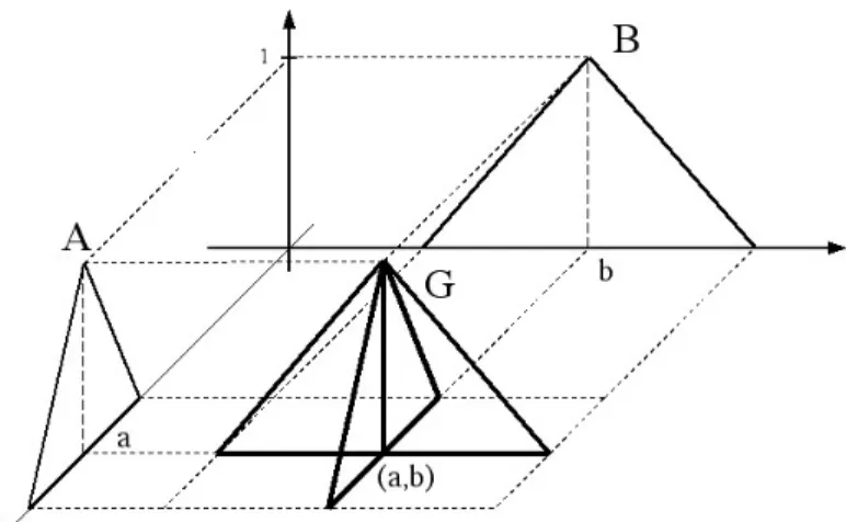
Definition 2.3. A fuzzy setAis called triangular fuzzy number with peak (or center)a, left widthα >0 and right widthβ >0if its membership function has the following form

A(t) =











1− a−t

α ifa−α≤t≤a 1− t−a

β ifa≤t≤a+β

0 otherwise

and we use the notationA= (a, α, β). It can easily be verified that

[A]^γ= [a−(1−γ)α, a+ (1−γ)β], ∀γ ∈[0,1].

The support ofA is(a−α, b+β). A triangular fuzzy number with centeramay be seen as a fuzzy quantity ”xis approximately equal toa”.

1

a

a-! a+"

4 1. Fuzzy Sets and Fuzzy Logic

[A]^γ= [a1(γ), a2(γ)].

The support ofAis the open interval (a1(0), a2(0)).

IfAis not a fuzzy number then there exists anγ∈[0,1] such that [A]^γ is not a convex subset ofR.

Fig. 1.2.Triangular fuzzy number.

Definition 1.1.4 A fuzzy setAis called triangular fuzzy number with peak (or center) a, left width α > 0 and right widthβ > 0 if its membership function has the following form

A(t) =









 1−a−t

α ifa−α≤t≤a 1−t−a

β ifa≤t≤a+β

0 otherwise

and we use the notationA= (a, α, β). It can easily be verified that [A]^γ= [a−(1−γ)α, a+ (1−γ)β], ∀γ∈[0,1].

The support ofAis(a−α, b+β). A triangular fuzzy number with centera may be seen as a fuzzy quantity

”xis approximately equal toa”.

Definition 1.1.5 A fuzzy setAis called trapezoidal fuzzy number with tolerance interval[a, b], left widthαand right widthβif its membership function has the following form

A(t) =









 1−a−t

α ifa−α≤t≤a 1 ifa≤t≤b 1−t−b

ifa≤t≤b+β

Figure 2.1: Triangular fuzzy number.

Definition 2.4. A fuzzy setAis called trapezoidal fuzzy number with tolerance interval[a, b], left width αand right widthβif its membership function has the following form

A(t) =











1− a−t

α ifa−α≤t≤a 1 ifa≤t≤b 1− t−b

β ifa≤t≤b+β

0 otherwise

and we use the notation

A= (a, b, α, β). (2.1)

It can easily be shown that[A]^γ= [a−(1−γ)α, b+ (1−γ)β]for allγ ∈[0,1]. The support ofAis (a−α, b+β).

8

(10)

1

a-! a b b+"

= (a, b, α, β). (1.1)

It can easily be shown that

[A]^γ= [a−(1−γ)α, b+ (1−γ)β], ∀γ∈[0,1].

The support ofAis(a−α, b+β).

Fig. 1.3.Trapezoidal fuzzy number.

A trapezoidal fuzzy number may be seen as a fuzzy quantity

”xis approximately in the interval [a, b]”.

Definition 1.1.6 Any fuzzy numberA∈ Fcan be described as

A(t) =









 L

%a−t α

&

ift∈[a−α, a]

1 ift∈[a, b]

R

%t−b) β

&

ift∈[b, b+β]

0 otherwise

where[a, b]is thepeakorcoreofA,

L: [0,1]→[0,1], R: [0,1]→[0,1]

are continuous and non-increasing shape functions withL(0) =R(0) = 1and R(1) =L(1) = 0. We call this fuzzy interval ofLR-type and refer to it by

A= (a, b, α, β)LR

The support ofAis(a−α, b+β).

Figure 2.2: Trapezoidal fuzzy number.

A trapezoidal fuzzy number may be seen as a fuzzy quantity ”x is approximately in the interval [a, b]”.

Definition 2.5. Any fuzzy numberA∈ F can be described as

A(t) =











L a−t α

!

ift∈[a−α, a]

1 ift∈[a, b]

R t−b) β

!

ift∈[b, b+β]

0 otherwise

where[a, b]is thepeakorcoreofA,L: [0,1]→[0,1]andR: [0,1]→[0,1]are continuous and non- increasing shape functions withL(0) =R(0) = 1andR(1) =L(1) = 0. We call this fuzzy interval of LR-type and refer to it byA= (a, b, α, β)LR. The support ofAis(a−α, b+β).

Definition 2.6. LetA= (a, b, α, β)LRbe a fuzzy number of typeLR. Ifa=bthen we use the notation

A= (a, α, β)LR (2.2)

and say thatAis a quasi-triangular fuzzy number. Furthermore ifL(x) =R(x) = 1−x, then instead ofA= (a, b, α, β)_LRwe writeA= (a, b, α, β).

Let A and B are fuzzy subsets of a classical set X 6= ∅. We say that A is a subset of B if A(t)≤B(t)for allt∈X. Furthermore,AandBare said to be equal, denotedA=B, ifA⊂Band B ⊂A. We note thatA=B if and only ifA(x) =B(x)for allx∈X. The intersection ofAandB is defined as

(A∩B)(t) = min{A(t), B(t)}=A(t)∧B(t), ∀t∈X.

The union ofAandBis defined as

(A∪B)(t) = max{A(t), B(t)}=A(t)∨B(t), ∀t∈X.

The complement of a fuzzy setAis defined as(¬A)(t) = 1−A(t),∀t∈X.

A fuzzy setr¯in the real line is said to be a fuzzy point, if its membership function is defined by

¯ r(z) =

( 1 ifz=r, 0 ifz6=r.

dc_817_13

(11)

That is,r¯is nothing else but the characteristic function of the singleton{r}.

Triangular norms were introduced by Schweizer and Sklar [131] to model distances in probabilistic metric spaces. In fuzzy sets theory triangular norms are extensively used to model logical connective and.

Definition 2.7. A mappingT: [0,1]×[0,1]→[0,1]is said to be a triangular norm (t-norm for short) iff it is symmetric, associative, non-decreasing in each argument andT(a,1) =a, for alla∈[0,1]. In other words, any t-normT satisfies the properties:

T(x, y) =T(y, x), ∀x, y∈[0,1] (symmetricity)

T(x, T(y, z)) =T(T(x, y), z), ∀x, y, z ∈[0,1] (associativity) T(x, y)≤T(x⁰, y⁰)ifx≤x⁰andy≤y⁰ (monotonicity) T(x,1) =x, ∀x∈[0,1] (one identy)

These axioms attempt to capture the basic properties of set intersection. The basic t-norms are:

• minimum (or Mamdani [126]):TM(a, b) = min{a, b},

• Łukasiewicz:T_L(a, b) = max{a+b−1,0}

• product (or Larsen [110]):TP(a, b) =ab

• weak:

T_W(a, b) =

( min{a, b} ifmax{a, b}= 1

0 otherwise

• Hamacher [99]:

H_γ(a, b) = ab

γ+ (1−γ)(a+b−ab), γ ≥0 (2.3) All t-norms may be extended, through associativity, ton > 2arguments. A t-normT is called strict ifT is strictly increasing in each argument. A t-normT is said to be Archimedean iffT is continuous andT(x, x)< xfor allx∈(0,1). Every Archimedean t-normT is representable by a continuous and decreasing functionf: [0,1]→ [0,∞]withf(1) = 0andT(x, y) =f⁻¹( min{f(x) +f(y), f(0)}).

The functionf is the additive generator ofT. A t-normT is said to be nilpotent ifT(x, y) = 0holds for somex, y∈(0,1). The operationintersectioncan be defined by the help of triangular norms.

Definition 2.8. LetT be a t-conorm. TheT-intersection ofAandBis defined as (A∩B)(t) =T(A(t), B(t)), ∀t∈X.

Triangular conorms are extensively used to model logical connectiveor.

Definition 2.9. A mappingS: [0,1]×[0,1] → [0,1]is said to be a triangular co-norm (t-conorm) if it is symmetric, associative, non-decreasing in each argument andS(a,0) = a, for alla ∈ [0,1]. In other words, any t-conormSsatisfies the properties:

S(x, y) =S(y, x) (symmetricity)

(12)

S(x, S(y, z)) =S(S(x, y), z) (associativity)

S(x, y)≤S(x⁰, y⁰)ifx≤x⁰andy≤y⁰ (monotonicity) S(x,0) =x, ∀x∈[0,1] (zero identy)

IfT is a t-norm then the equalityS(a, b) := 1−T(1−a,1−b), defines a t-conorm and we say thatSis derived fromT. The basic t-conorms are:

• maximum:S_M(a, b) = max{a, b}

• Łukasiewicz:S_L(a, b) = min{a+b,1}

• probabilistic:S_P(a, b) =a+b−ab

• strong:

ST RON G(a, b) =

( max{a, b} ifmin{a, b}= 0

1 otherwise

• Hamacher:

HOR_γ(a, b) = a+b−(2−γ)ab 1−(1−γ)ab , γ≥0 The operationunioncan be defined by the help of triangular conorms.

Definition 2.10. LetSbe a t-conorm. TheS-union ofAandBis defined as (A∪B)(t) =S(A(t), B(t)), ∀t∈X.

2.1 The extension principle

In order to use fuzzy numbers and relations in any intelligent system we must be able to perform arithmetic operations with these fuzzy quantities. In particular, we must be able to toadd,subtract,multiply anddividewith fuzzy quantities. The process of doing these operations is calledfuzzy arithmetic. we will first introduce an important concept from fuzzy set theory called theextension principle. We then use it to provide for these arithmetic operations on fuzzy numbers. In general the extension principle pays a fundamental role in enabling us to extend any point operations to operations involving fuzzy sets. In the following we define this principle.

Definition 2.11(Zadeh’s extension principle, [153]). AssumeX andY are crisp sets and letf be a mapping fromX toY,f:X → Y, such that for eachx ∈ X, f(x) = y ∈ Y. AssumeAis a fuzzy subset ofX, using the extension principle, we can definef(A)as a fuzzy subset ofY such that

f(A)(y) =

sup_x_∈_f−1(y)A(x) iff⁻¹(y)6=∅

0 otherwise (2.4)

wheref⁻¹(y) ={x∈X|f(x) =y}.

(13)

Iff(x) =λxandA∈ F then we will writef(A) =λA. Especially, ifλ=−1then we have (−1A)(x) = (−A)(x) =A(−x), x∈R.

It should be noted that Zadeh’s extension principle is nothing else but a straightforward generalization of set-valued functions (see [114] for details).

The extension principle can be generalized ton-place functions using the sup-min operator.

Definition 2.12(Zadeh’s extension principle forn-place functions, [153]). LetX₁, X₂, . . . , X_nandY be a family of sets. Assumef is a mapping

f:X₁×X₂× · · · ×X_n→Y, that is, for eachn-tuple(x1, . . . , x_n)such thatx_i∈X_i, we have

f(x1, x2, . . . , xn) =y ∈Y.

LetA₁, . . . , A_n be fuzzy subsets ofX₁, . . . , X_n, respectively; then the (sup-min) extension principle allows for the evaluation of f(A1, . . . , A_n). In particular, f(A1, . . . , A_n) = B, whereB is a fuzzy subset ofY such that

f(A1, . . . , An)(y) =

sup{min{A₁(x1), . . . , An(xn)} |x∈f⁻¹(y)} iff⁻¹(y)6=∅

0 otherwise. (2.5)

Forn= 2then the sup-min extension principle reads f(A₁, A₂)(y) = sup

f(x1,x2)=y{A₁(x₁), A₂(x₂)}.

Example 2.1. Letf:X×X→Xbe defined asf(x1, x₂) =x₁+x₂, i.e. f is the addition operator.

SupposeA1andA2are fuzzy subsets ofX. Then using the sup-min extension principle we get f(A₁, A₂)(y) = sup

x1+x2=ymin{A₁(x₁), A₂(x₂)} (2.6) and we use the notationf(A₁, A₂) =A₁+A₂.

Example 2.2. Letf:X×X →Xbe defined asf(x1, x2) =x1−x2, i.e. fis the subtraction operator.

SupposeA₁andA₂are fuzzy subsets ofX. Then using the sup-min extension principle we get f(A1, A₂)(y) = sup

x1−x2=ymin{A₁(x1), A2(x2)}, and we use the notationf(A1, A₂) =A₁−A₂.

The sup-min extension principle forn-place functions is also a straightforward generalization of set-valued functions. Namely, letf:X₁×X₂ → Y be a function. Then the image of a (crisp) subset (A₁, A₂)⊂X₁×X₂byf is defined by

f(A1, A₂) ={f(x1, x₂)|x₁ ∈Aandx₂ ∈A₂} and the characteristic function off(A1, A2)is

χ_f_(A₁_,A₂₎(y) = sup{min{χ_A₁(x), χ_A₂(x)} |x∈f⁻¹(y)}.

(14)

Then replacing the characteristic functions by fuzzy sets we get Zadeh’s sup-min extension principle forn-place functions (2.5).

Let A = (a1, a2, α1, α2)LR, and B = (b1, b2, β1, β2)LR, be fuzzy numbers of LR-type. Using the sup-min extension principle we can verify the following rules for addition and subtraction of fuzzy numbers of LR-type.

A+B = (a1+b1, a2+b2, α1+β1, α2+β2)LR

A−B= (a₁−b₂, a₂−b₁, α₁+β₂, α₂+β₁)_LR.

In particular ifA = (a1, a₂, α₁, α₂)andB = (b1, b₂, β₁, β₂)are fuzzy numbers of trapezoidal form then

A+B = (a₁+b₁, a₂+b₂, α₁+β₁, α₂+β₂) (2.7) A−B = (a1−b2, a2−b1, α1+β2, α2+β1). (2.8) IfA= (a, α₁, α₂)andB = (b, β₁, β₂)are fuzzy numbers of triangular form then

A+B = (a+b, α₁+β₁, α₂+β₂), A−B = (a−b, α₁+β₂, α₂+β₁) and ifA= (a, α)andB = (b, β)are fuzzy numbers of symmetric triangular form then

A+B = (a+b, α+β), A−B = (a−b, α+β), λA= (λa,|λ|α).

LetA andB be fuzzy numbers with[A]^α = [a1(α), a2(α)]and[B]^α = [b1(α), b2(α)]. Then it can easily be shown that

[A+B]^α= [a₁(α) +b₁(α), a₂(α) +b₂(α)], [A−B]^α= [a₁(α)−b₂(α), a₂(α)−b₁(α)],

[λA]^α=λ[A]^α,

where[λA]^α = [λa1(α), λa2(α)]ifλ≥0and[λA]^α = [λa2(α), λa1(α)]ifλ <0for allα ∈[0,1], i.e. anyα-level set of the extended sum of two fuzzy numbers is equal to the sum of theirα-level sets.

We note here that from sup

x1−x2=ymin{A₁(x1), A2(x2)}= sup

x1+x2=ymin{A₁(x1), A2(−x₂)},

it follows that the equalityA₁−A₂ =A₁+ (−A₂)holds. HoweverA−Ais defined by the sup-min extension principle as

(A−A)(y) = sup

x1−x2=ymin{A(x1), A(x2)}, y ∈R which turns into

[A−A]^α= [a1(α)−a2(α), a2(α)−a1(α)], which is generally not a fuzzy point.

Theorem 2.1(Nguyen, [129]). Letf:X → Xbe a continuous function and letAbe fuzzy numbers.

Then

[f(A)]^α =f([A]^α)

wheref(A)is defined by the extension principle (2.4) andf([A]^α) ={f(x)|x∈[A]^α}.

(15)

If[A]^α= [a₁(α), a₂(α)]andf is monoton increasing then from the above theorem we get [f(A)]^α=f([A]^α) =f([a1(α), a2(α)]) = [f(a1(α)), f(a2(α))].

Theorem 2.2(Nguyen, [129]). Letf:X×X→Xbe a continuous function and letAandBbe fuzzy numbers. Then

[f(A, B)]^α=f([A]^α,[B]^α), where

f([A]^α,[B]^α) ={f(x1, x2)|x1 ∈[A]^α, x2 ∈[B]^α}.

Letf(x, y) =xyand let[A]^α = [a1(α), a2(α)]and[B]^α = [b1(α), b2(α)]be two fuzzy numbers.

Applying Theorem 2.2 we get

[f(A, B)]^α =f([A]^α,[B]^α) = [A]^α[B]^α. However the equation

[AB]^α= [A]^α[B]^α= [a1(α)b1(α), a2(α)b2(α)]

holds if and only ifAandBare both nonnegative, i.e. A(x) =B(x) = 0forx≤0.

2.2 Fuzzy implications

Ifp is a proposition of the form ”x isA” whereAis a fuzzy set, for example, ”big pressure” and q is a proposition of the form ”yisB” for example, ”small volume” then one encounters the following problem: How to define the membership function of the fuzzy implication A → B? It is clear that (A→B)(x, y)should be definedpointwisei.e.(A→B)(x, y)should be a function ofA(x)andB(y).

That is(A→B)(u, v) =I(A(u), B(v)). We shall use the notation(A→B)(u, v) =A(u)→B(v).

In our interpretationA(u)is considered as the truth value of the proposition ”uis big pressure”, and B(v)is considered as the truth value of the proposition ”vis small volume”.

uis big pressure→vis small volume≡A(u)→B(v)

One possible extension of material implication to implications with intermediate truth values is A(u)→B(v) =

( 1 ifA(u)≤B(v) 0 otherwise This implication operator is calledStandard Strict.

”4 is big pressure”→ ”1 is small volume”=A(4)→B(1) = 0.75→1 = 1.

However, it is easy to see that this fuzzy implication operator is not appropriate for real-life applications.

Namely, letA(u) = 0.8andB(v) = 0.8. Then we have

A(u)→B(v) = 0.8→0.8 = 1.

Let us suppose that there is a small error of measurement or small rounding error of digital computation in the value ofB(v), and instead 0.8 we have to proceed with 0.7999. Then from the definition of Standard Strict implication operator it follows that

A(u)→B(v) = 0.8→0.7999 = 0.

(16)

This example shows that small changes in the input can cause a big deviation in the output, i.e. our system is very sensitive to rounding errors of digital computation and small errors of measurement.

A smoother extension of material implication operator can be derived from the equation X→Y = sup{Z|X∩Z ⊂Y},

where X, Y and Z are classical sets. Using the above principle we can define the following fuzzy implication operator

A(u)→B(v) = sup{z|min{A(u), z} ≤B(v)} that is,

A(u)→B(v) =

1 ifA(u)≤B(v) B(v) otherwise

This operator is calledG¨odelimplication. Using the definitions of negation and union of fuzzy subsets the material implicationp→q =¬p∨qcan be extended by

A(u)→B(v) = max{1−A(u), B(v)} This operator is calledKleene-Dienesimplication.

In many practical applications one uses Mamdani’s implication operator to model causal relationship between fuzzy variables. This operator simply takes the minimum of truth values of fuzzy predi- cates

A(u)→B(v) = min{A(u), B(v)}

It is easy to see this is not a correct extension of material implications, because0 → 0 yields zero.

However, in knowledge-based systems, we are usually not interested in rules, in which the antecedent part is false. There are three important classes of fuzzy implication operators:

• S-implications: defined by

x→y=S(n(x), y)

whereSis a t-conorm andnis a negation on[0,1]. These implications arise from the Boolean formalism

p→q =¬p∨q.

Typical examples ofS-implications are the Łukasiewicz and Kleene-Dienes implications.

• R-implications: obtained by residuation of continuous t-normT, i.e.

x→y= sup{z∈[0,1]|T(x, z)≤y}

These implications arise from theIntutionistic Logicformalism. Typical examples ofR-implications are the G¨odel and Gaines implications.

• t-norm implications: ifT is a t-norm then

x→y=T(x, y)

Although these implications do not verify the properties of material implication they are used as model of implication in many applications of fuzzy logic. Typical examples of t-norm implications are the Mamdani (x→y= min{x, y}) and Larsen (x→y =xy) implications.

(17)

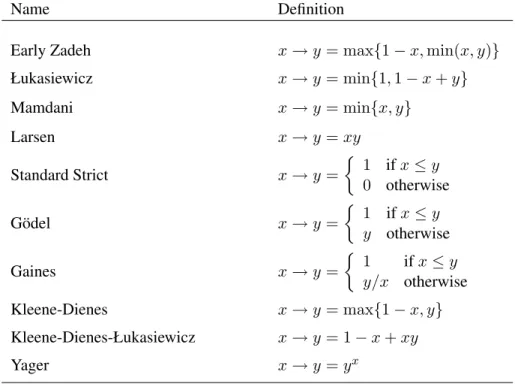
Name Definition

Early Zadeh x→y = max{1−x,min(x, y)}

Łukasiewicz x→y = min{1,1−x+y}

Mamdani x→y = min{x, y}

Larsen x→y =xy

Standard Strict x→y =

1 ifx≤y 0 otherwise

G¨odel x→y = 1 ifx≤y

y otherwise

Gaines x→y =

1 ifx≤y y/x otherwise

Kleene-Dienes x→y = max{1−x, y}

Kleene-Dienes-Łukasiewicz x→y = 1−x+xy

Yager x→y =y^x

Table 2.1: Fuzzy implication operators.

The use of fuzzy sets provides a basis for a systematic way for the manipulation of vague and imprecise concepts. In particular, we can employ fuzzy sets to represent linguistic variables. A linguistic variable can be regarded either as a variable whose value is a fuzzy number or as a variable whose values are defined in linguistic terms.

Definition 2.13. A linguistic variable is characterized by a quintuple (x, T(x), U, G, M)

in whichxis the name of variable;T(x)is the term set ofx, that is, the set of names of linguistic values ofxwith each value being a fuzzy number defined onU;Gis a syntactic rule for generating the names of values ofx; andM is a semantic rule for associating with each value its meaning.

For example, ifspeedis interpreted as a linguistic variable, then its term setT(speed) could be T ={slow, moderate, fast, very slow, more or less fast, sligthly slow, . . .}

where each term inT(speed) is characterized by a fuzzy set in a universe of discourseU = [0,100].

We might interpret

• slowas ”a speed below about 40 mph”

• moderateas ”a speed close to 55 mph”

• fastas ”a speed above about 70 mph”

(18)

These terms can be characterized as fuzzy sets whose membership functions are slow(v) =





1 ifv ≤40

1−(v−40)/15 if40≤v≤55

0 otherwise

moderate(v) =

1− |v−55|/30 if40≤v≤70

0 otherwise

fast(v) =









1 ifv≥70

1−70−v

15 if55≤v≤70

0 otherwise

In many practical applications we normalize the domain of inputs and use the following type of fuzzy partition: NVB (Negative Very Big), NB (Negative Big), NM (Negative Medium), NS (Negative Small), ZE (Zero), PS (Positive Small), PM (Positive Medium), PB (Positive Big), PVB (Positive Very Big). We will use the following parametrized standard fuzzy partition of the unit inteval. Suppose thatU = [0,1]

andT(x)consists ofK+ 1,K ≥2, terms,

T ={small₁, around 1/K, around 2/K, . . . , around (K-1)/K,big_K} which are represented by triangular membership functions{A1, . . . , AK+1}of the form

A₁(u) = [small₁](u) =

( 1−Ku if0≤u≤1/K

0 otherwise (2.9)

A_k(u) = [aroundk/K](u) =







Ku−k+ 1 if(k−1)/K≤u≤k/K k+ 1−Ku ifk/K ≤u≤(k+ 1)/K

0 otherwise

(2.10) for1≤k≤(K−1), and

A_K+1(u) = [big_K](u) =

( Ku−K+ 1 if(K−1)/K ≤u≤1

0 otherwise (2.11)

IfK = 1then the fuzzy partition for the [0,1] interval consists of two linguistic terms{small,big} which are defined by

small(t) = 1−t, big(t) =t, t∈[0,1]. (2.12) Suppose thatU = [0,1]andT(x)consists of2K+ 1,K ≥2, terms,

T ={small1, . . . ,smallK = small,big₀= big,big₁, . . . ,big_K} which are represented by triangular membership functions as

small_k(u) =





1−K

ku if0≤u≤k/K

0 otherwise

(2.13) fork≤k≤K,

big_k(u) =





u−k/K

1−k/K ifk/K≤u≤1

0 otherwise

(2.14) for0≤k≤K−1.

(19)

2.3 The theory of approximate reasoning

In 1979Zadehintroduced the theory of approximate reasoning [156]. This theory provides a powerful framework for reasoning in the face of imprecise and uncertain information. Central to this theory is the representation of propositions as statements assigning fuzzy sets as values to variables. Suppose we have two interactive variablesx ∈ X andy ∈ Y and the causal relationship between xandy is completely known. Namely, we know thaty is a function ofx, that isy =f(x). Then we can make inferences easily

”y =f(x)” & ”x=x₁”−→”y =f(x1)”.

This inference rule says that if we havey = f(x), for all x ∈ X and we observe thatx = x1 theny takes the valuef(x₁). More often than not we do not know the complete causal linkf betweenxand y, only we now the values off(x)for some particular values ofx, that is

<1: Ifx=x₁theny=y₁

<2: Ifx=x₂theny=y₂ . . .

<n: Ifx=x_ntheny=y_n

If we are given an x⁰ ∈ X and want to find an y⁰ ∈ Y which correponds tox⁰ under the rule-base

<={<1, . . . ,<m}then we have an interpolation problem.

Let x and y be linguistic variables, e.g. ”x is high” and ”y is small”. The basic problem of approximate reasoning is to find the membership function of the consequence C from the rule-base {<1, . . . ,<n}and the factA.

<1: ifxisA₁thenyisC₁,

<2: ifxisA₂thenyisC₂,

· · · ·

<n: ifxisA_nthenyisC_n

fact: xisA

consequence: yisC

In fuzzy logic and approximate reasoning, the most important fuzzy inference rule is theGeneralized Modus Ponens(GMP). The classicalModus Ponensinference rule says:

premise ifpthen q

fact p

consequence q

This inference rule can be interpreted as: If p is true andp → q is true then q is true. If we have fuzzy sets,A ∈ F(U)andB ∈ F(V), and a fuzzy implication operator in the premise, and the fact is also a fuzzy set,A⁰ ∈ F(U), (usually A 6= A⁰) then the consequnce, B⁰ ∈ F(V), can be derived from the premise and the fact using the compositional rule of inference suggested by Zadeh [154]. The Generalized Modus Ponensinference rule says

premise ifxisAthen yisB

fact xisA⁰

consequence: yisB⁰

(20)

where the consequenceB⁰is determined as a composition of the fact and the fuzzy implication operator B⁰ =A⁰◦(A→B), that is,

B⁰(v) = sup

u∈U

min{A⁰(u),(A→B)(u, v)}, v ∈V.

The consequenceB⁰ is nothing else but the shadow ofA→BonA⁰. The Generalized Modus Ponens, which reduces to classical modus ponens whenA⁰ =AandB⁰ =B, is closely related to the forward data-driven inference which is particularly useful in the Fuzzy Logic Control. In many practical cases instead of sup-min composition we use sup-t-norm composition.

Definition 2.14. LetT be a t-norm. Then the sup-T compositional rule of inference rule can be written as,

premise ifxisAthen yisB

fact xisA⁰

consequence: yisB⁰

where the consequenceB⁰is determined as a composition of the fact and the fuzzy implication operator B⁰ =A⁰◦(A→B), that is,

B⁰(v) = sup{T(A⁰(u),(A→B)(u, v))|u∈U}, v ∈V.

It is clear thatT can not be chosen independently of the implication operator.

Suppose thatA,BandA⁰ are fuzzy numbers. The GMP should satisfy some rational properties Property 2.1. Basic property:

if xisAthen yisB xisA

yisB Property 2.2. Total indeterminance:

if xisAthen yisB xis¬A

yisunknown Property 2.3. Subset:

if xisAthen yisB xisA⁰ ⊂A

yisB Property 2.4. Superset:

if xisAthen yisB xisA⁰

yisB⁰⊃B

(21)

Suppose thatA,BandA⁰are fuzzy numbers. The GMP with Mamdani implication inference rule says

if xisAthen yisB xisA⁰

yisB⁰ where the membership function of the consequenceB⁰is defined by

B⁰(y) = sup{A⁰(x)∧A(x)∧B(y)|x∈R}, y ∈R.

It can be shown that the Generalized Modus Ponens inference rule with Mamdani implication operator does not satisfy all the four properties listed above. However, it does satisfy all the four properties with G¨odel implication.

(22)

Chapter 3

OWA Operators in Multiple Criteria Decisions

The process of information aggregation appears in many applications related to the development of intelligent systems. In 1988 Yager introduced a new aggregation technique based on the ordered weighted averaging operators (OWA) [142]. The determination of ordered weighted averaging (OWA) operator weights is a very important issue of applying the OWA operator for decision making. One of the first approaches, suggested by O’Hagan, determines a special class of OWA operators having maximal entropy of the OWA weights for a given level of orness; algorithmically it is based on the solution of a constrained optimization problem. In 2001, using the method of Lagrange multipliers, Full´er and Majlender [84] solved this constrained optimization problem analytically and determined the optimal weighting vector. In 2003 using the Karush-Kuhn-Tucker second-order sufficiency conditions for opti- mality, Full´er and Majlender [86] computed the exact minimal variability weighting vector for any level of orness.

In 1994 Yager [145] discussed the issue of weightedminandmax aggregations and provided for a formalization of the process of importance weighted transformation. In 2000 Carlsson and Full´er [24] discussed the issue of weighted aggregations and provide a possibilistic approach to the process of importance weighted transformation when both the importances (interpreted as benchmarks) and the ratings are given by symmetric triangular fuzzy numbers. Furthermore, we show that using the possibilistic approach (i) small changes in the membership function of the importances can cause only small variations in the weighted aggregate; (ii) the weighted aggregate of fuzzy ratings remains stable under small changes in the nonfuzzy importances; (iii) the weighted aggregate of crisp ratings still remains stable under small changes in the crisp importances whenever we use a continuous implication operator for the importance weighted transformation.

In 2000 and 2001 Carlsson and Full´er [25, 30] introduced a novel statement of fuzzy mathematical programming problems and provided a method for finding a fair solution to these problems. Suppose we are given a mathematical programming problem in which the functional relationship between the decision variables and the objective function is not completely known. Our knowledge-base consists of a block of fuzzy if-then rules, where the antecedent part of the rules contains some linguistic values of the decision variables, and the consequence part consists of a linguistic value of the objective function. We suggested the use of Tsukamoto’s fuzzy reasoning method to determine the crisp functional relationship between the objective function and the decision variables, and solve the resulting (usually nonlinear) programming problem to find a fair optimal solution to the original fuzzy problem.

(23)

In this Chapter we first discuss Fullér and Majlender [84, 86] papers on obtaining OWA operator weights and survey some later works that extend and develop these models. Then following Carlsson and Fullér [24] we show a possibilistic approach to importance weighted aggregations. Finally, following Carlsson and Fullér [25, 30] we show a solution approach to fuzzy mathematical programming problems in which the functional relationship between the decision variables and the objective function is not completely known (given by fuzzy if-then rules).

3.1 Averaging operators

In a decision process the idea oftrade-offscorresponds to viewing the global evaluation of an action as lying between theworstand thebestlocal ratings. This occurs in the presence of conflicting goals, when a compensation between the corresponding compatibilities is allowed. Averaging operators realize trade-offs between objectives, by allowing a positive compensation between ratings. An averaging (or mean) operatorMis a functionM: [0,1]×[0,1]→[0,1]satisfying the following properties

• M(x, x) =x, ∀x∈[0,1], (idempotency)

• M(x, y) =M(y, x), ∀x, y∈[0,1], (commutativity)

• M(0,0) = 0,M(1,1) = 1, (extremal conditions)

• M(x, y)≤M(x⁰, y⁰)ifx≤x⁰andy≤y⁰(monotonicity)

• M is continuous

It is easy to see that ifM is an averaging operator then

min{x, y} ≤M(x, y)≤max{x, y}, ∀x, y∈[0,1]

An important family of averaging operators is formed by quasi-arithmetic means M(a1, . . . , an) =f⁻¹

1 n

Xn i=1

f(ai)

This family has been characterized by Kolmogorov as being the class of all decomposable continuous averaging operators. For example, the quasi-arithmetic mean ofa₁ anda₂is defined by

M(a1, a₂) =f⁻¹

f(a₁) +f(a₂) 2

.

The concept of ordered weighted averaging (OWA) operators was introduced by Yager in 1988 [142] as a way for providing aggregations which lie between the maximum and minimums operators.

The structure of this operator involves a nonlinearity in the form of an ordering operation on the elements to be aggregated. The OWA operator provides a new information aggregation technique and has already aroused considerable research interest [149].

(24)

Definition 3.1 ([142]). An OWA operator of dimension n is a mapping F: Rⁿ → R, that has an associated weighting vectorW = (w1, w₂, . . . , w_n)^T such asw_i ∈[0,1], 1≤i≤n, andw₁+· · ·+ wn= 1. Furthermore

F(a1, . . . , a_n) =w₁b₁+· · ·+w_nb_n= Xn j=1

w_jb_j, whereb_jis thej-th largest element of the bagha₁, . . . , a_ni.

A fundamental aspect of this operator is the re-ordering step, in particular an aggregate a_i is not associated with a particular weightw_ibut rather a weight is associated with a particular ordered position of aggregate. When we view the OWA weights as a column vector we will find it convenient to refer to the weights with the low indices as weights at the top and those with the higher indices with weights at the bottom. It is noted that different OWA operators are distinguished by their weighting function. In [142] Yager pointed out three important special cases of OWA aggregations:

• F^∗: In this caseW =W^∗ = (1,0. . . ,0)^T andF^∗(a1, . . . , an) = max{a1, . . . , an},

• F_∗: In this caseW =W_∗ = (0,0. . . ,1)^T andF_∗(a1, . . . , a_n) = min{a₁, . . . , a_n},

• F_A: In this caseW =W_A= (1/n, . . . ,1/n)^T andF_A(a1, . . . , a_n) = a1+· · ·+an

n .

A number of important properties can be associated with the OWA operators. we will now discuss some of these. For any OWA operatorF holds

F_∗(a₁, . . . , a_n)≤F(a₁, . . . , a_n)≤F^∗(a₁, . . . , a_n).

Thus the upper an lower star OWA operator are its boundaries. From the above it becomes clear that for anyF

min{a₁, . . . , a_n} ≤F(a1, . . . , a_n)≤max{a₁, . . . , a_n}.

The OWA operator can be seen to be commutative. Let ha1, . . . , ani be a bag of aggregates and let {d₁, . . . , d_n}be anypermutationof thea_i. Then for any OWA operatorF(a₁, . . . , a_n) =F(d₁, . . . , d_n).

A third characteristic associated with these operators ismonotonicity. Assumea_iandc_iare a collection of aggregates,i = 1, . . . , n such that for each i, a_i ≥ c_i. Then F(a1, . . . , a_n) ≥ F(c1, c₂, . . . , c_n), whereF is some fixed weight OWA operator. Another characteristic associated with these operators is idempotency. Ifa_i = afor allithen for any OWA operatorF(a1, . . . , a_n) = a. From the above we can see the OWA operators have the basic properties associated with anaveraging operator.