A GraphBLAS solution to the SIGMOD 2014 Programming Contest using multi-source BFS

A GraphBLAS solution to the SIGMOD 2014 Programming Contest using multi-source BFS

M´arton Elekes^∗, Attila Nagy^∗, D´avid S´andor^∗, J´anos Benjamin Antal, Timothy A. Davis^†, G´abor Sz´arnyas^∗‡

∗Budapest University of Technology and Economics, Department of Measurement and Information Systems

†Computer Science and Engineering, Texas A&M University, College Station, TX, USA

‡MTA-BME Lend¨ulet Research Group on Cyber-Physical Systems Email:elekes@mit.bme.hu,davis@tamu.edu,szarnyas@mit.bme.hu

Abstract—The GraphBLAS standard defines a set of funda- mental building blocks for formulating graph algorithms in the language of linear algebra. Since its first release in 2017, the expressivity of the GraphBLAS API and the performance of its implementations (such as SuiteSparse:GraphBLAS) have been studied on a number of textbook graph algorithms such as BFS, single-source shortest path, and connected components. However, less attention was devoted to other aspects of graph processing such as handling typed and attributed graphs (also known as property graphs), and making use of complex graph query techniques (handling paths, aggregation, and filtering). To study these problems in more detail, we have used GraphBLAS to solve the case study of the 2014 SIGMOD Programming Contest, which defines complex graph processing tasks that require a diverse set of operations. Our solution makes heavy use of multi-source BFS algorithms expressed as sparse matrix-matrix multiplications along with other GraphBLAS techniques such as masking and submatrix extraction. While the queries can be formulated in GraphBLAS concisely, our performance evaluation shows mixed results. For some queries and data sets, the performance is competitive with the hand-optimized top solutions submitted to the contest, however, in some cases, it is currently outperformed by orders of magnitude.

I. INTRODUCTION

Motivation.Since the release of GraphBLAS [20] in 2017, its applicability for graph analytical kernels has been studied in depth [17], [28], [9], [19], [30], including all six algorithms defined in the GAP Benchmark Suite [3]. While these efforts focused on algorithms defined on untyped graphs with no attributes (except edge weights for the shortest path algorithm), graphs with types and attributes received less attention. Such graphs, known asattributed graphs[24] orproperty graphs[1]

have gained popularity in recent years [23] by providing an intuitive data model for modelling complex interconnected systems such as social networks, telecommunications, and financial transactions. The property graph data model allows users to query their data using a rich set of operators including graph pattern matching, cycle detection, using relational oper- ators such as aggregation and filtering, running computations along paths, etc. Consequently, there is an increasing demand for graph databasescapable of storing and processing such data sets [5]. Still, as of today, there is no single system available that ensures good performance on a diverse set of graph operations. The reason behind this is threefold: (1) the difficulty to overcome the “curse of connectedness”, i.e. the inherently complex nature of graph data [25], (2) the lack

of a unified algebra for diverse graph queries, (3) the lack of sophisticated optimization methods [24] which consider the graph structure, its properties and their correlations [22].

We believe that the GraphBLAS API and its implementations have already made significant progress in tackling the first two problems and can be extended to tackle the last one.

Challenge. Integrating GraphBLAS into a property graph query engine necessitates overcoming a number of challenges including loading the graph, handling types and properties, performing computations on induced subgraphs, evaluating cyclic queries, computing aggregation and filtering operations, etc. To demonstrate some of these problems, we use the 2014 SIGMOD Programming Contest as a case study [8].¹The tasks of this contest are defined on a property graph and consist of complex graph queries involving a mix ofgraph algorithms (such as connected components),complex graph patterns (i.e.

basic graph patterns extended with relational-like features such as filtering), andnavigation[1].

Contribution.This paper presents a solution for the tasks of the 2014 SIGMOD Programming Contest. We formulated and implemented GraphBLAS algorithms for multiple BFS variants, including bidirectional and multi-source BFS.

Related systems. We are aware of two systems that use GraphBLAS to evaluate graph queries. RedisGraph [7] is a graph database that uses SuiteSparse:GraphBLAS to evaluate Cypher queries [13]. MAGiQ [14] is an RDF processing engine which maps SPARQL queries to linear algebra. Currently, neither of these systems supports workloads with queries as complex as the ones given in the programming contest.

Related contests. The 2018 Transformation Tool Contest’s

“Social Media” case required participants to solve two queries on a social network defined over a similar graph schema to the one in the SIGMOD 2014 contest. This contest focused on incremental evaluation and the complexity of the queries was limited. We gave a GraphBLAS solution for this in [12].

Structure.This paper is structured as follows. Sec. II describes the graph schema and the queries of the programming contest.

Sec. III outlines the GraphBLAS standard and its relevant constructs. Sec. IV shows our GraphBLAS-based building blocks, Sec. V presents our query implementations, and Sec. VI discusses the experimental results. Finally, Sec. VII concludes.

1https://www.cs.albany.edu/^∼sigmod14contest/

II. GRAPHSCHEMA ANDQUERIES

Graph schema. The social network instances used in the contest are represented as a property graph [1] over the schema shown in Fig. 1a. The edges in the graph are directed with the exception of theknows edges which are treated as undirected.

Data sets. Data sets are produced by the LDBC Datagen [22].

This generates realistic power-law degree distribution for the Person-knows-Person subgraph and introduces correlations and anti-correlations (e.g. people in neighbouring countries are more likely to become friends than people in distant countries).

Queries.The contest defines the following queries:

Q1. Shortest Distance over Frequent Communication Paths (Fig. 1b): Given two integer Person IDsp1andp2, and another integer x, find the minimum number of hops betweenp1andp2in the graph induced by Persons who both have made more thanxComments in reply to the other one’s Comments, and know each other.

Q2. Interests with Large Communities (Fig. 1c): Given an integerk and a birthday d, find the top-k Tags. A Tag is characterized with its range, i.e. the size of the largest connected component in the graph induced by Persons who are interested in that Tag, were born ondor later, and know each other.

Q3. Socialization Suggestion (Fig. 1d): Given an integerk, an integer maximum hop counth, and a Place namep, find the top-ksimilar pairs of Persons based on the number of common interest Tags. For each of thek pairs mentioned above, the two Persons must be located in p or study or work at Organisations in p. Furthermore, these two Persons must be no more than hhops away from each other in the originalknows graph.

Q4. Most Central People(Fig. 1e): Given an integerk and a Tag namet, find the top-kPersons based on thecloseness centrality value(CCV) in the graph induced by Persons who are members of Forums that have Tagt and know each other. For each Person,CCV(p) = ^(C(p)−1)_{(n−1)⋅s(p)}²,where C(p)is the size of the connected component of vertexp, s(p)is the sum of geodesic distances to all other reachable Persons from p, and n is the number of vertices in the induced graph. If the divisor is 0, the centrality is 0.

III. THEGRAPHBLAS

Goal.The goal of GraphBLAS is to create a layer of abstraction between the graph algorithms and the graph analytics frame- work, separating the concerns of the algorithm developers from those of the framework developers and hardware designers. To achieve this, it builds on the theoretical framework of matrix operations on arbitrary semirings [16], which allows defining graph algorithms in the language of linear algebra. To ensure portability, the GraphBLAS standard defines a C API that can be implemented on a variety of hardware including GPUs.

Data structures.A graph withnvertices can be stored as a square adjacency matrixA∈N^n×n, where rows and columns both represent vertices of the graph and element A(i, j) contains the number of edges from vertex i to vertex j. If

(a) Schema of the social network graphs. Only the relevant vertex, edge, and property types are shown.

(b)Q1($p1, $p2, $x)→shortest path length.

(c)Q2($k, $d)→$k tag names.

(d)Q3($k, $h, $place)→$k pairs of Person IDs p1∣p2 where p1<p2.

(e)Q4($k, $t)→$k Person IDs.

Fig. 1: Graph schema and queries.

GrBmethod name notation mxm matrix-matrix multiplication C⟨M⟩ =A⊕.⊗B vxm vector-matrix multiplication w⟨m⟩ =u⊕.⊗A mxv matrix-vector multiplication w⟨m⟩ =A⊕.⊗u eWiseAdd element-wise, C⟨M⟩ =A⊕B

set union of patterns w⟨m⟩ =u⊕v eWiseMult element-wise, C⟨M⟩ =A⊗B

set intersection of patterns w⟨m⟩ =u⊗v

extract

extract submatrix C⟨M⟩ =A(I,J) extract column vector w⟨m⟩ =A(∶, j) extract row vector w⟨m⟩ =A(i,∶) extract subvector w⟨m⟩ =u(I) extractElementextract scalar element s=A(i, j)

s=u(i) apply apply unary operator C⟨M⟩ =f(A)

w⟨m⟩ =f(u) select (GxB) apply select operator C⟨M⟩ =f(A, k)

w⟨m⟩ =f(u, k) reduce reduce to column vector w⟨m⟩ = [⊕jA(∶, j)]

reduce to scalar s= [⊕_ijA(i, j)]

transpose transpose C⟨M⟩ =A^⊺

build matrix from tuples C ↦ {I, J, X}

vector from tuples w ↦ {I, X}

extractTuples extract index/value arrays {I, J, X} ↦ A {I, X} ↦ u

TABLE I: GraphBLAS operations used in this paper (based on [10]). Notation:Matrices and vectors are typeset in bold, start- ing with uppercase (A) and lowercase (u) letters, respectively.

Scalars including indices are lowercase italic (s,i, j) while arrays are uppercase italic (X,I,J).⊕and⊗are addition and multiplication operators of an arbitrary semiring (defaulting to conventional arithmetic+ and×operators). Masks⟨M⟩and

⟨m⟩are used to selectively write to the result matrix/vector.

The complement of a mask⟨M⟩can be selected with⟨¬M⟩.

the graph is undirected, the matrix is symmetric. For graphs with edge types, edges of each type can be represented as a bipartite graph. For example, instances of the hasInterest edge type between Person and Tag vertices can be stored in a Boolean matrix with a row for each Person and a column for each Tag, HasInterest∈B∣persons∣×∣tags∣. Edge types that have the same source and target type are captured as square matrices, e.g. Knows∈B∣persons∣×∣persons∣.

Navigation. The fundamental step in GraphBLAS is the multiplication of an adjacency matrix with another matrix or vector over a selected semiring. For example, the operation HasMemberLOR.LAND IsLocatedIn computed over the

“logical or.logical and“semiring returns a matrix representing the Places where a Forum’s members are located in. Meanwhile, when computed over the conventional arithmetic “plus.times”

semiring, HasMember⊕.⊗IsLocatedInalso returns the number of such Persons. A traversal from a certain set of vertices can be expressed by using a boolean vector f (often referred to as thefrontier,wavefront, orqueue) and settingtrue values for the elements corresponding to source vertices. For example, for Forums f∈B^∣forums∣,f LOR.LAND HasMember returns the Persons who belong to any of the forums in f. The

BFS navigation step can also be captured using other semirings such as LOR.FIRST, where FIRST(x, y) = x; LOR.SECOND, where SECOND(x, y) = y; and ANY.PAIR, where ANY(x, y) returns eitherxory, andPAIR(x, y) =1 [11].

Notation. Table I contains the list of GraphBLAS operations used in this paper. Additionally, we use D= diag(I, n) to construct a diagonal matrix with D(i, i) =1 fori∈I. For a more detailed overview of GraphBLAS, see [16] and [17].

IV. BUILDINGBLOCKS INGRAPHBLAS A. Dense Vertex Relabelling

The vertices in the generated input graphs havesparse IDs, i.e. identifiers which can take any UINT64 value. To map a set of nsparse IDs todense IDs which take up consecutive values in the[0, n−1]range, we need to performdense vertex relabelling [27], also known as vertex permutation [4] and mapping from sparse to dense keys [21]. A straightforward way to implement this mapping from an array of sparse IDs sparseids is to create a sparse vector as follows:

mapping ↦ {sparseids,[0,1, . . . , n−1]}

Given a sparse IDs, the GraphBLAS extract element operation d = mapping(s) returns the corresponding dense ID d.

Meanwhile, mapping from a dense IDdto a sparse ID can be performed trivially with an array lookupsparseids[d].

Implementation.Sparse vectors in SuiteSparse:GraphBLAS are stored with their indices in increasing order, therefore this step requires a sorting operation. Then, lookups are executed using a binary search among the vector’s indices (of non-zero values). In the rest of the paper, we assume that identifiers have already been relabelled to dense.

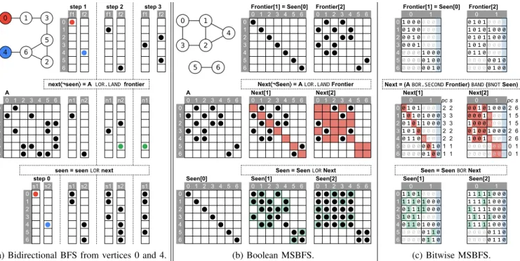
Algorithm 1 Bidirectional BFS algorithm.

1: procedureBIDIRECTIONALBFS(A, v1, v2) 2: Input:A∈B^n×n;v1, v2∈N

3: Data:frontier1,frontier2,next1,next2,seen1,seen2∈Bⁿ 4: Output:length∈N ▷length of unweighted shortest path 5: ifv1=v2then return0

6: frontier1,seen1 ↦ {[v1],[true]}

7: frontier2,seen2 ↦ {[v2],[true]}

8: forlevel=1to⌈n/2⌉do

9: next1⟨¬seen1⟩ =ALOR.LANDfrontier1 10: ifnext1is emptythen returnno path found

11: ifnext1LANDnext2is not emptythen return2×level−1 12: next2⟨¬seen2⟩ =ALOR.LANDfrontier2

13: ifnext2is emptythen returnno path found

14: ifnext1LANDnext2is not emptythen return2×level 15: seen1=seen1LORnext1

16: seen2=seen2LORnext2 17: frontier1=next1 18: frontier2=next2

B. Bidirectional Search

Both queries 1 and 3 requirebidirectional search: the former searches for the shortest path between two Persons (where each pair of Persons along the path edge satisfies a constraint on the number of interactions), while the latter looks for pairs of Persons who are at mosth hops away. Bidirectional search

step 1 step 2 step 3 f1 f2 f1 f2 f1 f2 0⬤

1 ⬤

2 ⬤

3 ⬤

4 ⬤

5 ⬤

6 ⬤

next⟨¬seen⟩ = A LOR.LAND frontier A0 1 2 3 4 5 6 n1 n2 n1 n2 n1

0 ⬤

1⬤ ⬤ ⬤

2 ⬤ ⬤ ⬤

3 ⬤ ⬤ ⬤

4 ⬤

5 ⬤ ⬤ ⬤ ⬤ ⬤

6 ⬤ ⬤ ⬤ ⬤

seen = seen LOR next step 0

s1 s2 s1 s2 s1 s2 s1

0⬤ ⬤ ⬤ ⬤

1 ⬤ ⬤ ⬤

2 ⬤

3 ⬤ ⬤

4 ⬤ ⬤ ⬤

5 ⬤ ⬤

6 ⬤ ⬤

(a) Bidirectional BFS from vertices 0 and 4.

Frontier[1] = Seen[0] Frontier[2]

0 1 2 3 4 5 6 0 1 2 3 4 5 6

0⬤ ⬤ ⬤

1 ⬤ ⬤ ⬤ ⬤

2 ⬤ ⬤ ⬤ ⬤

3 ⬤ ⬤ ⬤

4 ⬤ ⬤ ⬤

5 ⬤ ⬤

6 ⬤ ⬤

Next⟨¬Seen⟩ = A LOR.LAND Frontier

A Next[1] Next[2]

0 1 2 3 4 5 6 0 1 2 3 4 5 6 0 1 2 3 4 5 6

0 ⬤ ⬤ ⬤ ⬤ ⬤ ⬤

1⬤ ⬤ ⬤ ⬤ ⬤ ⬤ ⬤

2 ⬤ ⬤ ⬤ ⬤ ⬤ ⬤ ⬤

3⬤ ⬤ ⬤ ⬤ ⬤ ⬤

4 ⬤ ⬤ ⬤ ⬤ ⬤ ⬤

5 ⬤ ⬤

6 ⬤ ⬤

Seen = Seen LOR Next

Seen[0] Seen[1] Seen[2]

0 1 2 3 4 5 6 0 1 2 3 4 5 6 0 1 2 3 4 5 6

0⬤ ⬤ ⬤ ⬤ ⬤ ⬤ ⬤ ⬤ ⬤

1 ⬤ ⬤ ⬤ ⬤ ⬤ ⬤ ⬤ ⬤ ⬤ ⬤

2 ⬤ ⬤ ⬤ ⬤ ⬤ ⬤ ⬤ ⬤ ⬤ ⬤

3 ⬤ ⬤ ⬤ ⬤ ⬤ ⬤ ⬤ ⬤ ⬤

4 ⬤ ⬤ ⬤ ⬤ ⬤ ⬤ ⬤ ⬤ ⬤

5 ⬤ ⬤ ⬤ ⬤ ⬤

6 ⬤ ⬤ ⬤ ⬤ ⬤

(b) Boolean MSBFS.

Frontier[1] = Seen[0] Frontier[2]

0 1 0 1

01 0 0 00 0 0 0 0 1 0 10 0 0 0 10 1 0 00 0 0 0 1 0 1 0 1 0 0 0 20 0 1 00 0 0 0 0 1 0 1 1 0 0 0 30 0 0 10 0 0 0 1 0 1 00 0 0 0 40 0 0 01 0 0 0 0 1 1 00 0 0 0 50 0 0 00 1 0 0 0 0 0 00 0 1 0 60 0 0 00 0 1 0 0 0 0 00 1 0 0 Next = (A BOR.SECOND Frontier) BAND (BNOT Seen)

Next[1] Next[2]

0 1 pc s 0 1 pc s

00 1 0 10 0 0 02 2 0 0 1 0 1 0 0 02 6 11 0 1 0 1 0 0 03 3 0 0 0 10 0 0 01 5 20 1 0 1 1 0 0 03 3 1 0 0 00 0 0 01 5 31 0 1 00 0 0 02 2 0 1 0 0 1 0 0 02 6 40 1 1 00 0 0 02 2 1 0 0 10 0 0 02 6 50 0 0 00 0 1 01 1 0 0 0 0 0 0 0 00 1 60 0 0 00 1 0 01 1 0 0 0 0 0 0 0 00 1

Seen = Seen BOR Next

Seen[1] Seen[2]

0 1 0 1

01 1 0 10 0 0 0 1 1 1 1 1 0 0 0 11 1 1 0 1 0 0 0 1 1 1 1 1 0 0 0 20 1 1 1 1 0 0 0 1 1 1 1 1 0 0 0 31 0 1 10 0 0 0 1 1 1 1 1 0 0 0 40 1 1 0 1 0 0 0 1 1 1 1 1 0 0 0 50 0 0 00 1 1 0 0 0 0 00 1 1 0 60 0 0 00 1 1 0 0 0 0 00 1 1 0

(c) Bitwise MSBFS.

Fig. 2: Example BFS executions: bidirectional BFS and MSBFS algorithms. MSBFS algorithms start from all vertices.Notation:

∎blocked by mask ¬Seen(boolean) or by the0 bit inBNOT Seen(bitwise),∎new non-zero value/bit added,∎0-padding.

Algorithm 2 Boolean all-source MSBFS algorithm.

1: procedureBOOLEANMSBFS(A) 2: Input:A∈B^n×n

3: Data:

4: Frontier,Seen∈B^n×n ▷initialized to all vertices

5: Next∈B^n×n ▷initially empty

6: fork=0ton−1do ▷initialize diagonal matrix 7: I[k] =k, X[k] =true

8: Frontier,Seen ↦ {I, I, X}

9: forlevel=1ton−1do

10: Next⟨¬Seen⟩ =ALOR.LANDFrontier 11: ifNextis emptythenbreak

12: Frontier=Next

13: Seen=SeenLORNext

in GraphBLAS can be implemented as two alternating BFS traversals as shown in Alg. 1 and illustrated in Fig. 2a. To perform a search performed between vertices v1 andv2, we initialize two frontiervectors, each containing one non-zero value at position v₁ and v₂, respectively. In each iterationl, we advance the first frontier and check whether its intersection with the current (not yet advanced) state of the second frontier contains any elements. If so, we found a path of length2×l−1.

If not, we advance the second frontier and intersect it with the first frontier. If the intersection has any elements, we found a path of length2×l. If the new frontier is empty in either case, no path can be found between verticesv1 andv2.

C. Multi-Source Breadth-First Search

Boolean MSBFS. Highly-optimized multi-source BFS algo- rithms have been used by multiple teams in the programming contest [26], [15] to efficiently evaluate queries 3 and 4. In

Algorithm 3 Bitwise all-source MSBFS algorithm.Notation:

popcountis a unary operator that counts the number of bits in anUINT64value. Lines 18–21 compute the CCV (cf. Alg. 7).

1: procedureBITWISEMSBFS(A) 2: Input:A∈B^n×n

3: Data:

4: I, J, X∈UINT64ⁿ

5: Frontier,Next,Seen∈UINT64^{n×⌈n/64⌉}

6: sp∈Nⁿ,cpmo∈ [0,1]ⁿ ▷s(p), C(p) −1 7: Output:ccv∈ [0,1]ⁿ ▷closeness centrality values 8: fork=0ton−1do ▷initialize bit diagonal matrix 9: I[k] =k, J[k] =k/64, X[k] =1<< (64− (kmod 64)) 10: Frontier,Seen ↦ {I, J, X}

11: forlevel=1ton−1do

12: Next=ABOR.SECONDFrontier 13: Next⟨Next⟩BAND=BNOT(Seen)

14: Next=GxB NONZERO(Next) ▷prune explicit zeros 15: ifNextis emptythenbreak

16: Frontier=Next

17: Seen=SeenBORNext

18: nextCount= [⊕jpopcount(Next)(∶, j)]

19: sp⊕=nextCount×level

20: cpmo= [⊕_jpopcount(Seen)(∶, j)] −1 ▷C(p) −1 21: return(cpmo⊗cpmo) ⊘ ((n−1) ⊗sp) ▷^(C(p)−1)

2 (n−1)⋅s(p)

the GraphBLAS community, it is established that matrix- matrix multiplicationis a natural and efficient way to express MSBFS [29]. Using this idea, a GraphBLAS-based MSBFS algorithm is shown in Alg. 2 and illustrated in Fig. 2b.

Bitwise MSBFS.A key optimization among top-ranking teams was using bit arrays and bitwise manipulations to improve the performance of MSBFS. With the recent introduction of bitwise operators(e.g.GrB_BAND) in GraphBLAS v1.3 [6], it is

possible to use this optimization for MSBFS, shown in Alg. 3.

V. QUERIES

Query 1. Our implementation for Q1 (Alg. 4) first determines the induced subgraph. If the threshold xfor the number of interactions is −1, we use theKnows matrix, otherwise, we produce a matrix by traversing the hasCreatorandreplyOf edges, then filter for values larger than x. The length of the shortest path between the selected Persons is determined by running a bidirectional BFS (Alg. 1) on the induced subgraph.

Query 2. In Alg. 5, we first create a mask that corresponds to Persons born on dor later. We then iterate through each Tag (implemented as an outer OpenMP parallel for loop in our code), and determine Persons who are interested in said Tag and are kept by the mask. We extract theknowssubgraph and compute connected components using the FastSV algorithm [30], then determine the size of the largest component. Finally, we return the top-ktags based on their component size.

Query 3. In Alg. 6, we first compute the “local” Persons for the given place. The query requires us to determine pairs of Persons whose distance in the knows graph is at mosth hops. However, instead of evaluating the h-neighbourhood for each Person (which can get excessively large due to the exponential growth of the frontier), we look for “meeting vertices” (meetings) that are reachable from both Persons in at most ⌊h/2⌋ steps. Therefore, we initiate an MSBFS from all Persons (Lines 5–9) and run it for ⌊h/2⌋iterations. In the resulting Seenmatrix, rowirepresents the vertices reachable from Personi. A columnjwith more than one non-zero value captures a “meeting vertex”. For example, non-zero values in elementsSeen(x, j)andSeen(y, j)imply thatjis a meeting vertex between Persons x and y. We enumerate the pairs of Persons for each meeting vertex (concurrently) and store them in matrixCommonInt which represents the common interests of Persons. Finally, we return top-kmaximum values.

Since MSBFS steps move all frontiers simultaneously, special care needs to be taken for odd h values to ensure that the meeting vertex is at most ⌊h/2⌋steps from one local Person and ⌊h/2⌋ +1 steps from another one (yielding a total value of h). Therefore, once we performed the first⌊h/2⌋steps, we do an extra MSBFS step to advance the frontier and set the found elements to value 0.5 (Lines 10–12). Then, we filter for columns with a value larger than 1 (Line 13), thus omitting meeting vertices that only have two 0.5 values. Finally, we check the corresponding columns inSeenand only keep pairs of Persons whose summed values are larger than 1 (Line 16).

Query 4. Our solution for Q4 (Alg. 7) first navigates from the given Tagt to its Forums then to member Persons of such Forums. Then, it selects the corresponding rows/columns of the Knows matrix and computes the CCV values using a bitwise MSBFS algorithm (Alg. 3).

VI. EVALUATION

A. Benchmark Setup

Goal. We designed an experiment to compare the performance and scalability of our implementation against the top solutions.

Algorithm 4 Implementation of Q1 using Alg. 1.

1: Input:p1, p2∈N ▷target persons

2: x∈ {−1,0,1,2, . . .} ▷threshold

3: Output:l∈Z⁺ ▷length of the shortest path betweenp1 andp2 4: ifx= −1then

5: A=Knows 6: else

7: PA2Comment=HasCreator^⊺⊕.⊗ReplyOf 8: PA2PB⟨Knows⟩ =PA2Comment⊕.⊗HasCreator 9: A=GreaterThan(PA2PB, x)

10: A=ALANDA^⊺ ▷ensure thatxinteractions happened both ways 11: returnBIDIRECTIONALBFS(A, p1, p2)

Algorithm 5 Implementation of Q2. For CONNECTEDCOM-

PONENTS, we use the FastSV algorithm [30].

1: Input

2: k∈N, d∈Date ▷number of top-ktags, lower bound for birthdays 3: birthDay∈Date^{∣persons∣}

4: Output:[t1, . . . , tk] ∈N^k ▷top-ktags 5: birthDayMask=GreaterThanOrEq(birthDay, d)

6: fort=0to∣tags∣ −1do

7: interestedPerson⟨birthDayMask⟩ =HasInterest(∶, t) 8: {Pt, } =interestedPerson

9: Knows t=Knows(Pt, Pt)

10: component ids=CONNECTEDCOMPONENTS(Knows t) 11: scores[t] = (maxi∈component idscounti(component ids), t) 12: returntop-ktagstbased on theirscorefromscores

Algorithm 6 Implementation of Q3 using Alg. 2. The call GETPERSONSFORPLACE returns Persons for a given Place.

1: Input:place∈N, k∈N ▷place, number of top tags to return 2: Data:Frontier,Next∈B^n×n,Seen∈Q^n×n

3: Output:{(p1,1, p2,1), . . . ,(p1,k, p2,k)} ⊂N^k×N^k ▷top-kpairs 4: localPersons=GETPERSONSFORPLACE(place) ▷details omitted 5: Frontier,Seen=diag(localPersons, n)

6: forlevel=1to⌊h/2⌋do

7: Next⟨¬Seen⟩ =FrontierLOR.LANDKnows

8: Seen=SeenLORNext

9: Frontier=Next 10: ifhis an odd numberthen

11: Next⟨¬Seen⟩ =FrontierLOR.LANDKnows

12: Seen⟨Next⟩ =0.5 ▷mark the last frontier 13: meetings=GreaterThan([⊕_iSeen(i,∶)],1) ▷pruning 14: for alljwheremeetings(j)is non-zerodo

15: {I, X} ↦ Seen(∶, j)

16: for allpairs of person indicesp1, p2∈Iwherep1<p2do 17: ifX[p1] +X[p2] >1then

18: CommonInt(p1, p2) =0 ▷common interest count 19: CommonInt⟨CommonInt⟩ =HasInterest⊕.⊗HasInterest^⊺ 20: returntop-k(p1, p2)pairs wherep1<p2inCommonInt

Algorithm 7 Implementation of Q4 using Alg. 3.

1: Input:k∈N, t∈N ▷number of top persons to return, tag id 2: Output:l∈ [0,1] ▷closeness centrality value 3: {I, } = (HasTag(∶,t)LOR.LANDHasMember)

4: A=diag(I, n)LOR.LANDKnowsLOR.LANDdiag(I, n) 5: returnBITWISEMSBFS(A)

data set (#persons) 1k 10k 100k 1M total vertices 611 434 6 389 475 63 391 437 631 648 214 total edges 1 910 684 19 769 080 195 547 183 1 948 640 608

TABLE II: Number of entities in the input graphs.

Solutions.We implemented our solution in C++ using version v3.3.3 of SuiteSparse:GraphBLAS and the latest LAGraph library [19].² We compared our implementation against two solutions of the programming contest created by teams “AWFY”

(ranked 1st) and “blxlrsmb” (ranked 4th), updated for GCC 9.³ Data sets. We were unable to obtain the data sets used in the contest, therefore we generated similar ones using the LDBC SNB Datagen’s [22] 2014 version.⁴ The data set statistics are shown in Table II. We also implemented a parameter generator that produces query input parameters using uniform sampling.

Environment.We performed the experiments on a cloud virtual machine with 32 (logical) Intel Xeon Skylake CPU cores clocked at 2GHz, 120GB RAM, and SSD storage, running Ubuntu 20.04. We used the GCC 9.3.0 compiler. We ran each benchmark with 80 different parameters.

B. Analysis

Performance. We visualized the distribution of the execution times obtained during the experiments: load times are shown in Fig. 3a and computation times in Fig. 3b. Forload times, other solutions consistently outperform our solution. AWFY provides particularly fast loads (which can be attributed to its usage of advanced CSV loading techniques presented in [21]). However, forcomputation times, our solution is competitive for Q2 (often outperforming other solutions). It provides good performance for Q3 and Q4, staying within an order of magnitude compared to the other highly-optimized solutions. Our solution exhibits a bimodal distribution for Q1, which can be attributed to the configuration parameter x: forx> −1, computing the induced subgraph is expensive. The execution times of our solution for Q1 are noticeably longer than the competition’s due to precomputing the entire induced graph (instead of computing the relevant edges on-the-fly during traversal).

Conciseness.We characterized the conciseness of each solution using lines of C++ code: AWFY consisted of 9,800 lines, blxlrsmb used 6,500 lines, while our code used 3,500 lines.

Threats to validity.We remark that the solutions used in the experiments are 6+ years old and might be improved by further optimizations that were unavailable at the time of the contest.

We have updated the solutions to GCC 9 but did not apply any further optimizations nor did we contact their original authors.

VII. CONCLUSION ANDFUTUREWORK

We presented a concise GraphBLAS solution for the 2014 SIGMOD Programming Contest’s queries. Even though our code has no direct calls to low-level CPU instructions (unlike the top contest solutions), its computation performance for queries 2, 3, and 4 on large graphs is within 1–2 orders of

2https://github.com/ldbc/sigmod2014-pc-graphblas

3https://github.com/ftsrg/sigmod2014-pc-top-solutions

4https://github.com/ldbc/ldbc snb datagen/releases/tag/early2014

Q1 Q2 Q3 Q4

1k persons10k persons100k persons1M persons

0.01 0.1

0.1 1

0.1 1 10

10 100

Execution time [s]

tool AWFY blxlrsmb GraphBLAS

(a) Load times of the solutions.

Q1 Q2 Q3 Q4

1k persons10k persons100k persons1M persons

0.0001 0.001 0.01 0.1

0.0001 0.001 0.01 0.1 1

0.0001 0.001 0.01 0.1 1 10

0.0001 0.001 0.01 0.1 1 10 100 1000 10000

Execution time [s]

tool AWFY blxlrsmb GraphBLAS

(b) Computation times of the solutions.

Fig. 3: Execution times of queries.

magnitude to the top solutions. A limitation of our current solution is an expensive load step, which often takes longer the computation itself. For this reason, our solution works best in cases when multiple queries are performed on the same graph.

As future work, we plan to apply direction-optimization [2], also known as push/pull [28] to the bidirectional and MSBFS algorithms, and improve the load performance by using a concurrent hashmap such as Folklore [18].

ACKNOWLEDGEMENTS

The research has received funding from the EU ECSEL JU under the H2020 Framework Programme, JU grant nr. 826452 (Arrowhead Tools project) and from the partners’ national funding authorities. Davis would like to acknowledge NSF (1514406, 1835499), Intel, NVIDIA, IBM, Redis Labs, and MIT LL for their support. The authors would like to thank members of the GraphBLAS mailing list, Arnau Prat-P´erez, and Dean de Leo for discussions.

REFERENCES

[1] R. Angles, M. Arenas, P. Barcel´o, A. Hogan, J. L. Reutter, and D. Vrgoc.

Foundations of modern query languages for graph databases. ACM Comput. Surv., 50(5):68:1–68:40, 2017.

[2] S. Beamer, K. Asanovic, and D. A. Patterson. Direction-optimizing breadth-first search. InSC. IEEE/ACM, 2012.

[3] S. Beamer, K. Asanovic, and D. A. Patterson. The GAP Benchmark Suite.CoRR, abs/1508.03619, 2015. http://arxiv.org/abs/1508.03619.

[4] M. Besta and T. Hoefler. Survey and taxonomy of lossless graph compres- sion and space-efficient graph representations.CoRR, abs/1806.01799, 2018. http://arxiv.org/abs/1806.01799.

[5] M. Besta, E. Peter, R. Gerstenberger, M. Fischer, M. Podstawski, C. Barthels, G. Alonso, and T. Hoefler. Demystifying graph databases:

Analysis and taxonomy of data organization, system designs, and graph queries.CoRR, abs/1910.09017, 2019. http://arxiv.org/abs/1910.09017.

[6] A. Buluc¸, T. Mattson, J. E. Moreira, S. McMillan, and C. Yang. The GraphBLAS C API specification. Version 1.3.0, 2019. https://people.

eecs.berkeley.edu/^∼aydin/GraphBLAS API C v13.pdf.

[7] P. Cailliau, T. Davis, V. Gadepally, J. Kepner, R. Lipman, J. Lovitz, and K. Ouaknine. RedisGraph GraphBLAS enabled graph database. In GrAPL at IPDPS, pages 285–286. IEEE, 2019.

[8] G. A. Chernishev, V. Sevostyanov, K. Smirnov, and I. Shkuratov. On several social network analysis problems. In All-Russian Scientific Conference ”Digital libraries: Advanced Methods and Technologies, Digital Collections”, pages 234–242, 2014.

[9] T. A. Davis. Graph algorithms via SuiteSparse:GraphBLAS: Triangle counting and K-truss. InHPEC. IEEE, 2018.

[10] T. A. Davis. Algorithm 1000: SuiteSparse:GraphBLAS: Graph algorithms in the language of sparse linear algebra.ACM Trans. Math. Softw., 2019.

[11] T. A. Davis. User guide for SuiteSparse:GraphBLAS, version 3.3.3, 2020. https://people.engr.tamu.edu/davis/GraphBLAS.html.

[12] M. Elekes and G. Sz´arnyas. An incremental GraphBLAS solution for the 2018 TTC Social Media case study. 2020. GrAPL at IPDPS.

[13] N. Francis, A. Green, P. Guagliardo, L. Libkin, T. Lindaaker, V. Marsault, S. Plantikow, M. Rydberg, P. Selmer, and A. Taylor. Cypher: An evolving query language for property graphs. InSIGMOD, pages 1433–1445.

ACM, 2018.

[14] F. T. Jamour, I. Abdelaziz, Y. Chen, and P. Kalnis. Matrix algebra framework for portable, scalable and efficient query engines for RDF graphs. InEuroSys, pages 27:1–27:15. ACM, 2019.

[15] M. Kaufmann, M. Then, A. Kemper, and T. Neumann. Parallel array- based single- and multi-source breadth first searches on large dense graphs. InEDBT, 2017.

[16] J. Kepner et al. Mathematical foundations of the GraphBLAS. InHPEC.

IEEE, 2016.

[17] M. Kumar, J. E. Moreira, and P. Pattnaik. GraphBLAS: Handling performance concerns in large graph analytics. InCF, pages 260–267.

ACM, 2018.

[18] T. Maier, P. Sanders, and R. Dementiev. Concurrent hash tables: Fast and general(?)! ACM Trans. Parallel Comput., 5(4):16:1–16:32, 2019.

[19] T. Mattson, T. A. Davis, M. Kumar, A. Buluc¸, S. McMillan, J. E. Moreira, and C. Yang. LAGraph: A community effort to collect graph algorithms built on top of the GraphBLAS. InGrAPL at IPDPS, 2019.

[20] T. G. Mattson, C. Yang, S. McMillan, A. Buluc¸, and J. E. Moreira.

Graphblas C API: Ideas for future versions of the specification. In HPEC. IEEE, 2017.

[21] T. M¨uhlbauer, W. R¨odiger, R. Seilbeck, A. Reiser, A. Kemper, and T. Neumann. Instant loading for main memory databases. VLDB, 6(14):1702–1713, 2013.

[22] M. Pham, P. A. Boncz, and O. Erling. S3G2: A scalable structure- correlated social graph generator. InTPCTC, pages 156–172. Springer, 2012.

[23] S. Sahu, A. Mhedhbi, S. Salihoglu, J. Lin, and M. T. ¨Ozsu. The ubiquity of large graphs and surprising challenges of graph processing: Extended survey. VLDB J., 29(2):595–618, 2020.

[24] S. Sakr, S. Elnikety, and Y. He. G-SPARQL: A hybrid engine for querying large attributed graphs. InCIKM, pages 335–344, 2012.

[25] B. Shao, Y. Li, H. Wang, and H. Xia. Trinity graph engine and its applications. IEEE Data Eng. Bull., 40(3):18–29, 2017.

[26] M. Then, M. Kaufmann, F. Chirigati, T. Hoang-Vu, K. Pham, A. Kemper, T. Neumann, and H. T. Vo. The more the merrier: Efficient multi-source graph traversal. PVLDB, 8(4):449–460, 2014.

[27] M. Then, M. Kaufmann, A. Kemper, and T. Neumann. Evaluation of parallel graph loading techniques. InGRADES at SIGMOD. ACM, 2016.

[28] C. Yang, A. Buluc¸, and J. D. Owens. Implementing push-pull efficiently in GraphBLAS. InICPP, pages 89:1–89:11. ACM, 2018.

[29] C. Yang, A. Buluc¸, and J. D. Owens. GraphBLAST: A high- performance linear algebra-based graph framework on the GPU. CoRR, abs/1908.01407, 2019. http://arxiv.org/abs/1908.01407.

[30] Y. Zhang, A. Azad, and Z. Hu. FastSV: A distributed-memory connected component algorithm with fast convergence. InPP. SIAM, 2020.