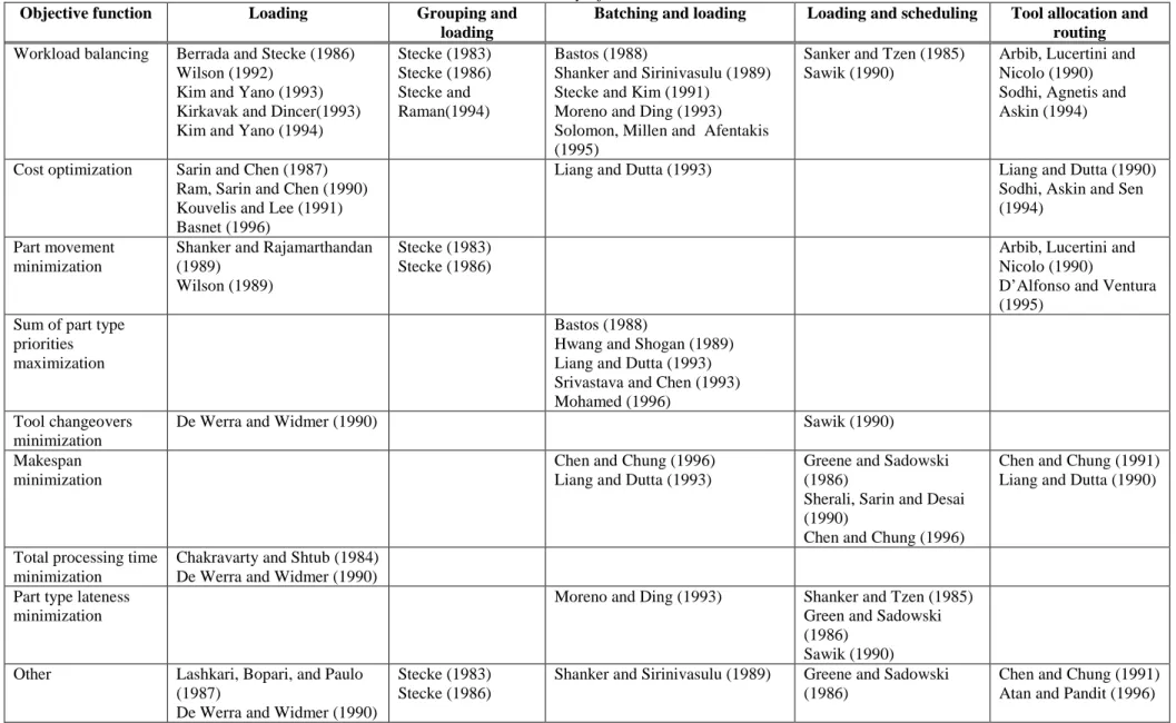
SENSITIVITY ANALYSIS AT PRODUCTION PLANNING AND PRODUCTION SCHEDULING MODELS
T
AMÁSK
OLTAI PH.D. IN ENGINEERINGBUDAPEST UNIVERSITY OF TECHNOLOGY AND ECONOMICS
DISSERTATION SUBMITTED IN PARTIAL FULFILLMENT OF THE REQUIREMENTS FOR THE TITLE OF D.SC. AT HUNGARIAN ACADEMY OF SCIENCES
BUDAPEST,2015
CONTENTS
1INTRODUCTION ... 1
2THE DIFFERENCE BETWEEN THE MANAGERIAL AND MATHEMATICAL INTERPRETATION OF SENSITIVITY ANALYSIS RESULTS IN LINEAR PROGRAMMING ... 5
2.1 Introduction ... 5
2.2 Basic definitions and concepts ... 6
2.3 Graphical illustration of the problem of sensitivity analysis ... 11
2.4 A practical approach to sensitivity analysis under degeneracy ... 16
2.5 Calculation of Type III sensitivity results of a production planning example ... 18
2.5.1 Sensitivity analysis of the right-hand side (RHS) elements ... 20
2.5.1 Sensitivity analysis of the objective function coefficients (OFCs) ... 21
2.6 Decreasing the number of additional LP problems ... 22
2.7 Conclusions of Chapter 2 ... 23
3ROUTE-INDEPENDENT ANALYSIS OF AVAILABLE CAPACITY IN FLEXIBLE MANUFACTURING SYSTEMS ... 25
3.1 Introduction ... 25
3.2 Illustration of the problem ... 26
3.3 Literature review ... 29
3.4 The requirement of an aggregation concept ... 29
3.5 Basic definitions and concepts of the aggregation based on operation types ... 32
3.6 Illustration of the available and extended capacity ranges ... 35
3.7 Model formulation ... 39
3.8 Sensitivity analyses of the operation type set constraints ... 42
3.8.1 Sensitivity of operation type set constraints to capacity requirements ... 42
3.8.2 Sensitivity of the operation type set constraints to machine capacity ... 44
3.9 Conclusions of Chapter 3 ... 46
4FORMULATION OF WORKFORCE SKILL CONSTRAINTS IN ASSEMBLY LINE BALANCING MODELS ... 48
4.1 Introduction ... 48
4.2 Formulation of the basic simple ALB models ... 50
4.3 Formulation of workforce skill constraints ... 53
4.3.1 Formulation of low-skill constraints (LSC) ... 54
4.3.2 Formulation of high-skill constraints (HSC) ... 55
4.3.3 Formulation of exclusive-skill constraints (ESC) ... 56
4.3.4 Summary of the suggested worker skill models ... 56
4.4 Application of simple ALB models with skill constraints at a bicycle manufacturer ... 58
4.4.1 Application of high-skill constraints (HSC) ... 62
4.4.2. Application of low-skill constraints (LSC) ... 62
4.5 Sensitivity analysis of line efficiency with respect to production quantity ... 63
4.6 The effect of the change of task times ... 65
4.6.1 The effect of the variation of task times ... 65
4.6.1 The influence of the learning effect ... 66
4.7 Conclusions of Chapter 4 ... 68
II 5APPLICATION OF PERTURBATION ANALYSIS FOR SENSITIVITY ANALYSIS OF A PRODUCTION
SCHEDULE ... 70
5.1 Introduction ... 70
5.2 Basic concepts of perturbation analysis (PA) ... 71
5.3 Formal treatment of perturbation analysis ... 71
5.3.1 Analysis of the NI and FO events ... 72
5.3.2 Generation of perturbations ... 75
5.3.3 Perturbation propagation ... 75
5.3.4 Calculation of the validity range of deterministic similarity ... 75
5.4 Gradient of the mean waiting time in the queue ... 77
5.5 Convergence properties of the gradient estimates ... 78
5.6 Computational results ... 78
5.6.1 Implementation of gradient calculation with PA in discrete event simulation ... 78
5.6.2 Implementation of gradient calculation when a production schedule is given ... 83
5.7 Conclusions of Chapter 5 ... 86
6SENSITIVITY OF A PRODUCTION SEQUENCE TO INVENTORY COST CALCULATION METHODS IN CASE OF A SINGE RESOURCE,DETERMINISTIC SCHEDULING PROBLEM ... 87
6.1 Introduction ... 87
6.2 Minimization of inventory holding cost with common due dates ... 89
6.2.1 Optimal schedule when interest is not compounded ... 90
6.2.2 Optimal schedule when interest is continuously compounded ... 91
6.2.3 Comparison of the optimal sequences ... 92
6.3 Extension of the calculation for different due dates of jobs ... 94
6.3.1 Optimal schedule when delivery dates are different and interest is not compounded ... 94
6.3.2 Optimal schedule when delivery dates are different and interest is continuously compounded ... 94
6.3.3 Comparison of the optimal sequences ... 95
6.4 Illustration of the results with the help of a calendar manufacturing process ... 96
6.5 Conclusions of Chapter 6 ... 98
7SUMMARY OF THE DISSERTATION ... 100
8 LIST OF PUBLICATIONS RELATED TO SCIENTIFIC RESULTS ... 102
8.1 List of pear reviewed journal papers related to scientific results ... 102
8.2 List of published conference papers related to the scientific results ... 103
8.3 List of other publications related to the scientific results ... 104
9LITERATURE ... 106
LIST OF TABLES
Table 2.1 Summary of notation of Chapter 2
Table 2.2 Shadow prices and validity ranges of the optimal values Table 2.3 Shadow prices and validity ranges at the optimal bases B1
Table 2.4 Shadow prices and validity ranges at the optimal bases B2
Table 2.5 Increase of the objective function by a unit of the increment of RHS elements Table 2.6 Objective function coefficient sensitivities and rate of changes at the optimal
bases B1
Table 2.7 Objective function coefficient sensitivities and rate of changes at the optimal bases B2
Table 2.8 Summary of additional LP problems for sensitivity analysis Table 2.9 Data of the sample production planning model
Table 2.10 Sensitivity analysis of the RHS elements Table 2.11 Sensitivity analysis of the OFCs
Table 3.1 Basic data of the sample problem (operation times in capacity units) Table 3.2 Summary of literature review
Table 3.3 Summary of notation of Chapter 3
Table 3.4 Definition of sets S′ and S″ in the sample problem
Table 3.5 Test results of different size problems (Lingo 6.0 solver, Pentium IV processor) Table 3.6 Comparison of problem sizes
Table 3.7 Sensitivity of operation type set constraints to capacity requirements of operation types (α=β=0.25)
Table 3.8 Sensitivity of the operation typeset constraints to machine capacity (α=β=0.25) Table 4.1 Summary of notation of Chapter 4
Table 4.2 Summary of ALB models and skill constraints
Table 4.3 Tasks and precedence relations of the sample bicycle model Table 4.4 Optimal solutions of the SALB models
Table 4.5 Summary of simulation results Table 5.1 Summary of notation of Chapter 5 Table 5.2 Results of a single simulation run
Table 5.3 Comparison of difference calculation and gradient estimation Table 5.4 Basic data of the FMS routing sample problem
Table 5.5 Gradient information at θ1,1=0.25, θ2,1=1 Table 5.6 Calculation steps of sensitivity analysis Table 5.7 Break of sequence sensitivity table Table 6.1 Summary of notation of Chapter 6
Table 6.2 Optimality conditions of the i–j sequence of jobs
Table 6.3 Inventory holding cost of different production schedules (Euros)
IV LIST OF FIGURES
Figure 2.1 Graphical illustration of the prototype problem
Figure 2.2 Graphical illustration of the modified prototype problem Figure 2.3 Implementation of sensitivity analysis
Figure 3.1 Illustration of the routing of part type i Figure 3.2 Activity based costing in a FMS
Figure 3.3 Allocation of operation types to machines
Figure 3.4 Illustration of the ideal available capacity range and the capacity requirements (α=0.25, β=0.25, x1=100, x2=20)
Figure 4.1 Precedence diagram of the sample problem Figure 4.2 Precedence graph of a sample bicycle
Figure 4.3 Effect of production quantity on line efficiency Figure 4.4 Illustration of bottleneck shift.
Figure 5.1 Illustration of no-input Figure 5.2 Illustration of full-output
Figure 5.3 Illustration of potential no-input Figure 5.4 Illustration of potential full-output Figure 5.5 Illustration of the overtake possibility
Figure 5.6 Implementation of perturbation analysis in discrete event simulation Figure 5.7 Transfer line example with three resources
Figure 5.8 FMS sample problem
Figure 5.9 Throughput as a function of routing parameters
Figure 5.10 The throughput and the ∂TP0/∂θ1,1-∂TP0/∂θ1,2 values in the θ2,1=1 cuts Figure 5.11 The throughput and the ∂TP0/∂θ2,1-∂TP0/∂θ2,2 values in the θ2,1=1 cuts Figure 5.12 Queuing network representation of the steel casting process
Figure 5.13 Sensitivity analysis of the break of sequence Figure 6.1 Illustration of the residence time of job i Figure 6.2 Interchange of job i and job j
Figure 6.3 Transformed exponential operation time function (q=0.6)
Figure 6.4 The f(t) function for the parameters of the calendar manufacturer (q=0.1092)
1 INTRODUCTION
The economical operation of production and service systems has always been a major concern of engineers. In 1886, Henry Towne of the Yale and Towne Company in a paper titled
“Engineer as an Economist” recommended that a new section should be organized within the American Society of Mechanical Engineers (ASME). This new section could be a forum for those professionals, who are mechanical engineers, but interested in the economic aspects of production (Towne, 1886). The recommendation of Towne initiated the rapid development of a new branch of engineering, which is called industrial engineering (IE) (Hicks, 1977). The official definition of industrial engineering formulated by the Institute of Industrial Engineering (IIE) states (Salvendy, 1992) that
“Industrial engineering is concerned with the design, improvement and installation of integrated systems of people, materials, information, equipment and energy. It draws upon specialized knowledge and skill in the mathematical, physical and social sciences together with the principles and methods of engineering analysis and design, to specify, predict, and evaluate the results to be obtained from such systems.”
The problems, scientific foundations and information processing infrastructure of IE have changed considerably since the time of Towne. By now, all stages of the lifecycle of production systems − design, implementation, operation, improvement and restructuring − are influenced by industrial engineering. The problems discussed in the dissertation are related to planning and scheduling of production operations. Production planning and production scheduling determines the allocation of manufacturing resources to production task on the medium and short run, that is, a plan should be prepared a priori, to determine how much and when to produce of the different parts/products, and what amount of resources should be applied during production. In the course of production, the difference of the plan and the actual operation must be compared, analyzed, and appropriate control actions are to be implemented if required.
The solution of the complicated problems of production planning and control is supported by operations research methods. Frequently, optimization models are formulated to determine the best possible production plan and production schedule. By the time of implementation or during operation several parameters − which were used to obtain the implemented solution − may change. Some of these changes are important and require actions on behalf of the decision maker. Other changes, however, may not influence the implemented decision, although influence the result of operation. Consequently, the robustness of the plan, that is, the sensitivity of the results with respect to some model parameters is important information for management decision-making (see for example, Little, 1970; Ragsdale, 2007;
Monostori et al., 2010).
Sensitivity analysis methods can be applied to get information about the effect of parameter changes on an optimal or on a heuristic solution. The objective of sensitivity analysis is to determine the effect of the change of parameters or conditions assumed in the planning phase on some performance measures important for decision-making. The method used for generating sensitivity information depends on the planning model, on the changing factor (parameter, condition) and on the performance measure.
Sometimes, calculating the value of the objective function with the original and with the changed values of a parameter, and analyzing the difference may lead to general sensitivity conclusions. One of the first, widely documented sensitivity analysis applied in industrial engineering has been the examination of the robustness of the classical economic order quantity (EOQ) formula in inventory management, which dates back to 1913 (Harris, 1913).
2 This analysis is based on the examination of the total cost function when some parameters (order cost, inventory holding rate) change, and the results are discussed in most of the basic production management related university textbooks (see for example, Nahmias, 1993;
Anderson, 1994; Waters, 1996).
The simple analysis of the change of the objective function value, however, may not always be sufficient to get proper sensitivity information. Sometimes, studying the structure of the problem may lead to analytical description of robustness and sensitivity. In linear programming, for example, the simplex method provides information about the sensitivity of the objective function and about the validity range of this sensitivity. This information is provided by the simplex table of the optimal solution (see for example Hillier and Lieberman, 1996; Prékopa, 1968). In case of discrete event simulation, perturbation analysis can be used to obtain sensitivity information related to a performance measure from a single sample path (Ho and Cao, 1991).
Frequently, in complex models, numerical examination of the behavior of an objective function in a predefined parameter range must be performed. Such analysis, however, requires extensive computations and advanced information processing environment.
No matter which technique is applied, information about sensitivity is important for the decision maker due to the following three reasons:
− Some model parameters may change despite of the intention of the decision maker. For example, a customer demand may change, an operation cost may increase or production capacity may decrease by the time a production plan is implemented. The operation manager must know whether the change of operation is required or the change of the parameters does not influence the plan, consequently, the change of operation is not necessary.
− The decision maker may have the possibility to change some parameters. For example, a selling price can be changed, a production capacity can be increased by overtime or a new production route of a part can be implemented. Analysis of the possible effects of these parameter changes is required before decision on implementation is made.
− Sometimes model parameters may change but the change of operation is not possible even if it were required. In these cases, the analysis of the consequences of the change helps to determine how far the actual operation is from the optimum, and what measures should be taken to avoid the unfavorable effects in the future.
The proper presentation of sensitivity information for management decision-making is also a very important question. Generally, sensitivity results consist of a large amount of data.
The range information of a linear programming solution contains the sensitivity range of several thousand objective function coefficients and shadow prices. Filtering and clustering this information is necessary for efficient decision-making. Graphical presentation of these data might considerably direct the attention of the decision maker to critical points, and highlights the most efficient intervention areas (Eschenbach, 1992).
Consequently, sensitivity analysis is important from theoretical and from practical points of view as well, and a strong emphasis is made to develop both theory and technique to obtain sensitivity information in several production related fields (see for example Wagner, 1995;
Saltelli, Tarantola and Campolongo, 2000; Higle and Wallace, 2003 or Hall and Posner, 2004;
Kövesi, 2011).
The application of sensitivity information to improve decision-making is not just a possibility, but also a necessity. The development of the theory and technology of data mining has a strong impact on production related decisions as well (Jackson, 2002). The information obtained by the processing of a large amount of data can be a source of competitive advantage according to Davenport (2006). If these data are efficiently collected (about customer behavior, about operation, about environmental conditions, etc.), if proper (statistical, operational research) methods are used to process these data, and the results are adequately
channeled into the decision-making process, then the competitors can be outperformed. The emphasis on the collection of a large amount of data and on the efficient processing of the collected information forms the basis of a new paradigm in management decision-making which is called competing on analytics (Davenport, 2006; Davenport and Harris, 2007;
Koltai, 2007).
The support of competition with the results of the processing of a large amount of data is possible as a consequence of the development of information technology. Data can be collected automatically about the progress of a production or a service process at reasonably low cost and with acceptable speed. The collected data can be processed with efficient and easy to use statistical and operation research software even on an ordinary computer.
Consequently, competing on analytics and big data management is becoming a general approach when decision support systems are designed (Davenport 2013).
On the one hand, the availability of a large amount of data about actual operation, and the possibilities of advanced data processing environment provide excellent opportunities for generating sensitivity information. On the other hand, sensitivity information is constantly demanded in a system which strives for continuous improvement of its operation.
The dissertation discusses the theoretical and practical aspects of sensitivity analysis results related to production planning and scheduling problems. In some cases, the derivation and analysis of sensitivity results of existing models are the main objective of the research. In other cases, new models are formulated and sensitivity analysis supports the application of the models. The following research problems are discussed in details in the dissertation:
1) Linear Programming (LP) is frequently applied to solve production planning problems.
The sensitivity information of the optimal plan with respect to the model parameters is important information for capacity extension, operation improvement and customer related decisions. In case of degenerate optimal solution, however, sensitivity information generated by the traditional LP solvers can be misleading. I have investigated the reason of the misleading sensitivity results and the ways of correcting this information.
2) In flexible manufacturing systems (FMS), products/parts can be manufactured by visiting different machines, that is, the same part may follow several different routes in the manufacturing process. Routing influences the available capacity of the system. Frequently, however, capacity related decisions must be made before parts are assigned to the specific routes. I have investigated how capacity of FMSs can be determined before the routing information is available, and I have analyzed the sensitivity of the results with respect to some basic model parameters.
3) In case of assembly lines, frequently, 0-1 mathematical programming models are used to allocate tasks to workstations. One important shortcoming of assembly line balancing (ALB) models is that the models do not take into consideration several real life conditions.
One important group of such conditions is related to workforce skills. I have developed a general framework to formulate workforce skill constraints. I have also investigated the effect of the change of production quantity on the optimal solution.
4) Scheduling problems of production systems are frequently solved with the help of discrete event simulation. The sensitivity of the scheduling criteria to the change of some model parameters is important information for the decision maker. I have analyzed the sensitivity of the throughput time and the sensitivity of waiting time with respect to some operation times, and I have determined the validity of these gradient information using perturbation analysis.
5) Frequently, the objective of scheduling is the minimization of inventory holding cost.
There are, however, several ways to determine the value of inventory holding cost. I have investigated how the optimal schedule of a single resource scheduling problem is influenced by the method of inventory holding cost calculation. I have also analyzed the robustness of
4 the optimal schedule using analytical and numerical methods as well.
Some remarks must be made about the structure and the content of this work.
− Each chapter of the dissertation is related to sensitivity analysis, however, the problems examined, the techniques used for modeling, and the generation of sensitivity information is different in each chapter. Consequently, a different method of notation is required in each chapter. To facilitate the reading of the text, each main chapter has a separate list of notation.
− The results of the main chapters have already been published in relevant scientific journals of the related areas. The content of the main chapters of this work is an edited and integrated version of the corresponding papers. Since these papers were written in the last 20 years, new results, algorithms, software and computing technology may have appeared. Those chapters which are based on earlier papers may not reflect the most up-to date technology, but the scientific results of the chapters are independent of the changes of the technological conditions and of the change of information technology.
2 THE DIFFERENCE BETWEEN THE MANAGERIAL AND MATHEMATICAL INTERPRETATION OF SENSITIVITY ANALYSIS RESULTS IN LINEAR PROGRAMMING
One important problem of production planning is the allocation of production resources to production tasks. This problem is frequently solved by mathematical programming models.
Linear programming (LP) has a special role within mathematical programming, because resource allocation problems can be easily described or efficiently approximated by linear relationships. The theory and practice of linear programming is well established and several software are available to support real life applications. The main result an LP problem is the optimal solution. In a production planning context the optimal solution determines the optimal allocation of production resources to production tasks. Further results of an LP problem are related to the sensitivity analysis of the optimal solution. In some cases LP sensitivity analysis results of the currently available LP solvers provide misleading information. In this chapter the problems of LP sensitivity information are explained, a new categorization of sensitivity information is provided and a calculation framework is suggested. The results of this chapter are based on the papers of Koltai and Terlaky (2000), Koltai and Tatay (2008) and Koltai and Tatay (2011).
2.1 Introduction
Linear programming (LP) is one of the most extensively used operations research technique in production and operations management (Johnson and Montgomery, 1974; Cane and Parker, 1996). As a result of the development of computer technology and the rapid evolution of user friendly LP software every operation manager can run an LP software easily and quickly on a laptop computer. Although to solve LP models is now accessible for everybody, the interpretation of the results requires a lot of skill. Most of the management science and operational research textbooks pay a special attention to sensitivity analysis, and to the problems of degeneracy, but sensitivity analysis under degeneracy is rarely discussed.
Commercially available software do not give enough information to the user about the existence and about the consequences of these, very common, special cases. In practice, managers very frequently misinterpret the LP results which may lead to erroneous decisions and to important financial and/or strategic disadvantages.
Several papers have addressed this issue. Evans and Baker (1982) draw the attention to the consequences of the misinterpretation of sensitivity analysis results in decision-making.
They illustrate their point with a simple example and list some published cases in which the erroneous interpretation of sensitivity analysis results is obvious. Aucamp and Steinberg (1982) also warn that shadow price analysis is incorrect in many textbooks, and that the shadow price is not equal to the optimal solution of the dual problem when the obtained optimal solution is degenerate. They present some examples of shadow price calculations by commercial packages. Akgül (1984) refines the shadow price definition of Aucamp and Steinberg, and introduces the negative and positive shadow prices for the increase and for the decrease of the right-hand side (RHS) elements. Greenberg (1986) shows that very frequently practical LP models have a netform structure; and netform structures are always degenerate.
He illustrates sensitivity analysis of netform type models by one of the Midterm Energy Market Model of the U.S. Department of Energy. Gal (1986) summarizes most of the critics concerning sensitivity analysis of LP models and highlights some important research directions. Rubin and Wagner (1990) illustrate the traps of the interpretation of LP results by using the industry cost curve model in a tutorial type paper written for managers and
6 instructors. Jansen, et al. (1997) explains the effect of degeneracy on sensitivity analysis by using a transportation model, and presents the shortcomings of the most frequently used LP packages. Wendell also pays special attention to correct and practically useful calculation of sensitivity information (see for example Wendell, 1985 and Wendell, 1992). The problem is not that operations researchers are unaware of the difficulties of sensitivity analysis. This issue is discussed thoroughly in the scientific literature, (see for example Gal, 1979; and Wendell, 1992) and a complete, mathematically correct treatment of sensitivity analysis is presented e.g. in Jansen et al. (1997), and in Roos at al. (1997). Practice, however, shows that the problem is not widely known among LP users, and available commercial software packages are not helping to recognize the difficulties.
The main objective of this chapter is to explain the difference between the managerial questions and the traditional mathematical interpretation of sensitivity analysis. In the first part of this chapter the basic definitions are introduced, the most important types of sensitivity information are classified, and degenerate LP solutions are illustrated graphically. Next, a production planning problem is used to demonstrate the consequences of incorrect interpretations of the provided sensitivity information. In the second part of the chapter a practice oriented framework for calculating sensitivity information is provided and sensitivity information for management decision-making are presented for a degenerate production planning problems. Finally, some recommendations are formulated both for decision makers and for software developers. All notations used in this chapter are summarized in Table 2.1.
2.2 Basic definitions and concepts
Every LP problem can be written in the following standard form,
{
c xAx b x 0}
x = ; ≥
min T (2.1)
where A is a given J x I matrix with full row rank and where the column vector b represents the right-hand side (RHS) terms and the row vector cT represents the objective function coefficients. Problem (2.1) is called the primal problem and a vector x≥0 satisfying Ax=b is called a primal feasible solution. The objective is to determine those values of the vector x which minimize the objective function. To every primal problem (1) the following problem is associated,
{
b yA y c}
y T T ≤
max (2.2)
Problem (2.2) is called the dual problem and a vector y satisfying ATy≤c is called a dual feasible solution. For every primal feasible x and dual feasible y it holds that cTx≥bTy and the two respective objective function values are equal if and only if both solutions are optimal (see for example Hillier and Liberman, 1995).
Most computer programs to solve linear programming problems are based on a version of the simplex method. Modern, hi-performance packages are furnished with interior point solvers as well; however, the implemented sensitivity analysis is based always on the simplex method. The simplex procedure selects a basis of the matrix A in every step The selected basis solution is calculated and the optimality criteria are checked. To define the optimal basis solution some preparation is needed.
Let B be a set of m indices, and AB be the matrix obtained by taking only those columns of A whose indices are in B. If AB is a nonsingular matrix then by using the vector xB=AB–1b a basis solution can be defined as
( )
=
otherwise.
0
,
∈B i xi xB i if
(2.3)
Table 2.1 Summary of notation of Chapter 2 Subscripts:
i − index of the variables of a primal LP problem (i=1,…,I), j − index of the variables of a dual LP problem (j=1,…,J),
t − index of the time period in the production planning example (t=1,…,T) n − index of the products in the production planning example (n=1, …,N).
Parameters:
A – coefficient matrix with elements aji,
AB − coefficient matrix containing only the columns of A in the basis, b – right-hand side vector with elements bj,
c – objective function coefficient vector with elements ci,
cB − objective function coefficients belonging to the variables in the basis, ei – unit vector with I elements, and with ei=1 and ek=0 for all k≠i, ej – unit vector with J elements, and with ej=1 and ek=0 for all k≠j, δ – perturbation of a right-hand side parameter
nt – number of working days in month t Dnt – demand of product n in period t,
pnt – unit production cost of product n in period t, hnt – unit inventory holding cost of product n in period t, Ct – production capacity in period t,
Wt – warehouse capacity in period t.
Sets:
B − index set containing the indices of the basis variables.
Variables:
x – variable vector of the primal problem with elements xi, xB – vector of the basis variables with elements (xB)i, x* – optimal solution of the primal problem with elements xi
*, y – variable vector of the dual problem with elements yj, y* – optimal solution of the dual problem with elements yj
* , s − slack variable vector with elements sj,
OF* – optimal value of the objective function, yj
– – the left shadow price of right-hand side element bj (δ<0), yj
+ – the right shadow price of right-hand side element bj (δ>0), γi – change of objective function coefficient ci,
γi
– – feasible decrease of objective function coefficient ci, γi
+ – feasible increase of objective function coefficient ci, ξj – change of right-hand side element bj,
ξj
– – feasible decrease of right-hand side element bj, ξj
+ – feasible increase of right-hand side element bj, nξj
– – feasible decrease of bj belonging to the left shadow price, nξj
+ – feasible increase of bj belonging to the left shadow price, pξj
– – feasible decrease of bj belonging to the right shadow price, pξj
+ – feasible increase of bj belonging to the right shadow price, xnt – production quantity of product n in period t,
Int – inventory of product n in period t.
8 If in addition xB≥0 holds then x is called a primal feasible basic solution. The variables with their index in B are the basic variables; the others are the non-basic variables. Dual variables can be associated to any basis AB as follows:
( )
AB cBy= −1T (2.4)
If c−ATy≥0 then y is a feasible solution for the dual problem, and y is called dual feasible basic solution. If the basis AB is both primal and dual feasible, then AB is an optimal basis, and the corresponding basic solutions x and y are optimal basis solutions for the primal and for the dual problems respectively. It might happen that a basis gives an optimal primal solution, but the related dual basis solution is dual infeasible. Such a basis is called primal optimal. Analogously, when a basis gives a dual optimal solution, but the related primal solution is infeasible, then the basis is called dual optimal.
Sometimes the optimal basis is not unique, more than one basis may yield an optimal solution either for the primal or for the dual problem or for both. This is called degeneracy and occurs very frequently in practice. Formally, a basis is called primal degenerate when there are variables with zero value among the basis variables and it is called dual degenerate when some dual slack variables si=ci−(ATy)i, not belonging to the basis indices B, are zero. In general, if a basis is either primal, or dual, or from both sides degenerate then we simply say that it is degenerate. In case of degeneracy many optimal solutions exists that are not basic solutions.
Very frequently the main parameters of an LP model changes (e.g. cost coefficients, resource capacities, etc.) and it would be important to know if any action on behalf of the decision maker is required as a consequence of these changes. Sensitivity analysis can help to answer this question if it is applied correctly. The objective of sensitivity analysis is to analyze the effect of the change of the objective function coefficients (OFC) and the effect of the change of the right-hand side (RHS) elements on the optimal value of the objective function, furthermore, the validity ranges of these effects. Depending on how this analysis is performed three types of sensitivities can be defined (Koltai and Terlaky, 1999, 2000):
− Type I sensitivity: Type I sensitivity determines those values of some model parameters for which a given optimal basis remains optimal. Sensitivity analysis of the optimal basis for the OFC elements determines within which range of an OFC the current optimal basis remains optimal and what is the rate of change (directional derivative) of the optimal objective function value when the OFC changes within this range. In case of the RHS elements the question is, within which range a RHS element can change so that the current optimal basis stays optimal, and what is the rate of change (shadow price) of the optimal objective function value within the determined interval.
Type I sensitivity analysis is implemented in almost all commercial software packages. In case of primal degeneracy, however, several bases may belong to the same optimal solution yielding different ranges and rate of changes for the same parameter to different optimal basis.
In case of dual degeneracy many primal optimal solutions, and therefore, many different optimal basis may exist resulting in different intervals and rates of changes. From mathematical point of view the provided information is correct, because the question is the sensitivity of the given optimal basis, but, can be misleading for decision makers, if the given information is not interpreted correctly.
− Type II sensitivity: Type II sensitivity determines those values of some model parameters for which the positive variables in a given primal and dual optimal solution remain positive, and the zero variables remain zero, i.e. the same activities remain active.
More accurately, we have an optimal solution (not necessarily basis solution) x with its support set supp(x)={ ixi >0}. We are looking for those model parameters, for which an optimal solution (basis or not basis) exists with precisely the same support set. Sensitivity
analysis of a given optimal solution for an OFC determines within which range of the OFC an optimal solution with the same support set exists and what is the rate of change (directional derivative) of the optimal objective function value when the OFC changes within this range.
In case of the RHS elements the question is, within which range a RHS element can change without the change of the support set of the optimal solution, and what is the rate of change (shadow price) of the optimal objective function value within the determined interval.
Contrary to Type I sensitivity, Type II sensitivity depends on the produced optimal solution, but not on which basis − if any − represents the given optimal solution.
− Type III sensitivity: Type III sensitivity determines those values of some model parameters for which the rate of change of the optimal value function is the same. Roughly speaking sensitivity (and range) analysis means the analysis of the effects of the change of some problem data, in particular an objective coefficient cj or right-hand side element bj. Let us assume that either ci+γi or bj+ξj is the perturbation. It is known that the optimal value function is a piecewise linear function of the parameter change (see for example Gal, 1979, Jansen et al., 1997 or Roos, Terlaky and Vial, 1997). In performing Type III sensitivity analysis one wants to determine the rate of the change of the optimal value function and the intervals within which the optimal value function changes linearly.
Type III sensitivity information is independent of the solution obtained, it depends only on the problem data and on which OFC or RHS element is changing.
The calculation and importance of the three different types of sensitivity information depends on the optimum solution produced by the LP solver. Most of the LP solvers used for small and medium size problems are based on some versions of the simplex method and they provide an optimal basis solution. Other solvers, typically used for (very) large scale problems are based on interior point methods and they provide an interior (i.e. strictly complementary) optimal solution. To distinguish among the three types of sensitivities is necessary because of the existence of degeneracy. The following cases can be observed:
− When the optimal solution is neither primal nor dual degenerate, then all the three types of sensitivities are the same, since there is a unique optimal solution with a unique optimal basis. In this case, the sensitivity analysis output of the available LP solvers provides reliable, useful information for decision-making.
− When the optimal solution is only primal degenerate then a unique primal optimal solution exists. Moreover, several optimal bases belong to the same, unique primal optimal solution. In this case Type I and Type II sensitivities may be different since there are different Type I sensitivity information for all the optimal basis. One important case is when the increase and the decrease of a RHS parameter results in different rate of changes, i.e. the optimal value function at the current point is not differentiable. Due to this fact the introduction of the right side and left side shadow prices and their respective sensitivities (Aucamp and Steinberg, 1982) was needed. Type II and Type III sensitivity information for the RHS elements are split into two parts: the left and right side sensitivities. The left and right linearity intervals of the optimal value function provide the Type III information. When the left and right side shadow prices are identical, then only one interval is given. Type II and Type III sensitivity information for an OFC are identical in the case when the solution is only primal degenerate.
− When the optimal solution is only dual degenerate, then several different primal optimal basis and non-basis solutions may exist with different support sets, while the dual optimal solution is unique. In this case Type I and Type II sensitivities at each alternative primal optimal basic solution are identical, but Type II sensitivities can be calculated from non-basic solutions as well. Type II sensitivity is interested only in the optimal solutions belonging to the same support sets, therefore, Type III sensitivity may be different from the Type II sensitivities of each optimal solution.
10
− When the optimum is both primal and dual degenerate, then all the three types of sensitivities may be different. In this case each optimal basis of each optimal basis solution may have a different Type I sensitivity information. Optimal solutions with different support sets may have different Type II sensitivities and can be examined at non-basis solutions as well. As it is known, Type III sensitivity information is uniquely determined; it is independent of the optimal solution obtained. Typically, the intervals provided by Type I and Type II sensitivities are subintervals of the Type III sensitivity intervals. The rates of changes produced by Type I and Type II either coincide with Type III information or are useless, their validity (as a sub-differential) is restricted to the current point only.
− In case of large models, solvers based on interior point methods (IPMs) are frequently used. IPM solvers generally provide strictly complementary optimal solutions. In this case Type I sensitivity cannot be asked because, in case of degeneracy, the produced optimal solution is not a basis solution. When one is interested in obtaining an optimal basis solution, a basis identification procedure might be applied to produce an optimal basis. Such procedures are implemented in many software packages. Type II and Type III sensitivity information are identical in this case, because the change of the support set of a strictly complementary optimal solution is in one to one correspondence with the linearity intervals of the optimal value function (Roos, Terlaky and Vial, 1997).
An important question is, when the difference between Type II and Type III sensitivities is important for the decision maker. When the decision maker implements an optimal solution then, in many situations, the important information is the sensitivity of the implemented optimal solution (Type II sensitivity). For example if an optimal production plan, determined by LP, is already running, then the important question is how the change of certain costs, or the change of a machine capacity influences the implemented plan. When the question is, how much a RHS element can be increased with the same consequences, and independently of the possible change of an optimal solution, then it is a Type III sensitivity question. For example if a machine capacity can be increased economically at the calculated shadow price, the decision maker should know how much the capacity can be increased economically in total. It is possible that different production plans (different optimal solutions, especially when optimal basis solutions are implemented) belong to different amount of capacity increases, but all capacity extensions are made at the same marginal benefits.
Type I sensitivity analysis is the classical sensitivity analysis, provided by most LP solvers. Type III sensitivity analysis examines the sensitivity of the decision criteria, and provides the widest range for the possible change of the parameter. Type II sensitivity analysis examines the sensitivity of an important property of the optimal operation. In this case the sensitivity range provided by Type III sensitivity is narrowed down with constraints expressing the required property of the optimal solution.
As a summary it can be stated that in case of degeneracy commercial packages do not provide the sensitivity information useful for the decision maker (note that in practice l problems are very frequently degenerate). They give answer to a less ambitious question.
They provide information about the interval of a parameter value within which the current optimal basis remains optimal, and at what rate the change of the parameter varies the optimal objective function value in that interval (Type I sensitivity). This answer is intimately related to the optimal basis obtained by the simplex solver. In case of degeneracy many different optimal bases exist, thus many different ranges and rates of changes might be obtained. To obtain the true Type III sensitivity information about the change of the value of the OFC and RHS elements one needs extra effort. In fact one has to solve some subsidiary LP=s for determining linearity intervals, and left and right derivatives of the optimal value function (see Chapter 2.4).
2.3 Graphical illustration of the problem of sensitivity analysis
When the LP problem has no more than two variables then the solution space and all the information concerning the optimum and its sensitivity, can be represented in a two dimensional space. The following problem will be our prototype problem (Koltai and Terlaky, 2000),
0 ,
≥0
≤ 500 L2
≤ 400 L1
≤ 1000 2
C2
≤ 600 C1
10 12
max
2 1
2 1
2 1
2 1
2 1
≥ + + +
x x
x x
x x
x x
x x
(2.5)
The feasible set and the solution of problem (2.5) can be seen on Figure 2.1.
Figure 2.1 Graphical illustration of the prototype problem
The two constraints (C1 and C2) and the upper bounds on x1 and x2 (L1 and L2) are represented as half spaces. The boundary of these spaces with the corresponding labels is depicted on the figure. The intersection of these half spaces is represented as a shaded area, which contains all the primal feasible solutions. The objective function (iso-profit line) is drawn as a straight dashed line. The objective function touches the shaded area at point P3, therefore the unique optimal solution is at x1=400 and x2=200.
In order to transform problem (2.5) into the standard form, indicated by problem (2.1), slack variables (denoted by si, i=1,...,4) are introduced for all the constraints, and the objective function is changed to have a minimization problem. The problem in standard form is as follows,
C1
C2 L1
L2
0 200 400 600 800 1000 1200
0 200 400 600 800
x2
x1
P3
P4 P0
P1 P2
12 0
, 0 , 0 , 0 , 0 , 0
500 :
L2
400 :
L1
1000 2
: C2
600 :
C1
10 12
min
4 3 2 1 2 1
4 2
3 1
2 2
1
1 2
1
2 1
≥
≥
≥
≥
≥
≥
= +
= +
= +
+
= +
+
−
−
s s s s x x
s x
s x
s x
x
s x
x
x x
(2.6)
Problem (2.6) shows that A is a 4x6 matrix with rank equal to 4. The values of the slack variables at P3 are the following,
s1=0; s2=0; s3=0; s4=300.
Since at P3 there are three nonzero variables (x1, x2 and s4) and the rank of matrix A is 4, the optimal solution is degenerate. This can be seen in Figure 2.1. The point P3 is the intersection of three lines (C1, C2 and L1). Two lines would be enough to determine the location of a point in a two dimensional space, therefore P3 is over determined. Even if we remove any one of C2, or L1, the point P3 remains the only optimal solution. This over determination of the optimal point is a graphical illustration of primal degeneracy.
Let us see the consequences of degeneracy on sensitivity analysis. The shadow prices and the corresponding validity ranges for the optimal solution, calculated with the help of Figure 2.1, are given in Table 2.2. The change of a RHS element is represented by a parallel shift of the corresponding line in Figure 2.1.
Table 2.2 Shadow prices and validity ranges of the optimal values Dual
variable
Current RHS value
Left side shadow
price
Validity range Right side shadow
price
Validity range
LL UL LL UL
yC1 600 10 400 600 8 600 750
yC2 1000 2 700 1000 0 1000 ∞
yL1 400 2 100 400 0 400 ∞
yL2 500 0 200 500 0 500 ∞
If the RHS of any of these constraints are decreased, then the left side shadow prices are obtained for each constraint respectively (column three of Table 2.2). The optimal point P3 is at the intersection of constraints C1, C2 and L1. The decrease of any of the RHS of these constraints results in the move of the optimum point, P3, which consequently changes the objective function value as well. Since the change of the RHS of L2 does not affect the location of P3 its shadow price is zero. C1 can be moved to P4, C2 and L1 can be moved to P2 with the same shadow price value. L2 can be moved to P3 without affecting the objective function value. The corresponding lower limits (LL) are given in the fourth column of Table 2.2. In case of left side shadow prices the upper limits (UL) are equal to the current values of the RHS elements (fifth column of Table 2.2).
If the RHS of any of these constraints are increased, then the right side shadow prices are obtained for each constraint, respectively (column six of Table 2.2). In case of constraints C2 and L2 the increase of the right-hand side values do not affect the location of the optimum point, because C1 and either C2 or L1 fixes its place. Therefore the corresponding right side shadow prices are equal to zero. When the right-hand side of C1 is increased, then the optimum point will stay at the intersection of C1 and C2 and the shadow price will be equal to 8. Since L2 does not affect the location of P3 its shadow price is also zero. In case of right side shadow prices the lower limits (LL) are equal to the current values of the RHS elements, while the upper limits (UL) are determined by the geometrical properties of the solution
space. When C1 is moved upward the intersection of C1 and C2 (P3) moves upward as well.
When P3 reaches L2, then the move of C1 does not affect the location of P3, and the shadow price turns into zero. The RHS value at this point is the UL of the sensitivity range, and it is equal to 750. The UL of all the other constrains are equal to infinity.
Table 2.3 shows the shadow prices and their validity ranges found by the STORM computer package (Emmons at al, 2001) at the optimal basis B1={1, 2, 3, 6}. It can be seen that at this basis the left side shadow prices and validity ranges were provided for constraints C1 and L1, and the right side shadow price and validity range was found for constraint C2.
Table 2.3 Shadow prices and validity ranges at the optimal bases B1 Dual
variable
Current RHS value
Left side shadow
price
Validity range
LL UL
yC1 600 10 400 600
yC2 1000 0 1000 ∞
yL1 400 2 100 400
yL2 500 0 200 ∞
Table 2.4 contains the shadow prices and their validity ranges found at the optimal basis B2={1, 2, 5, 6}. At this basis the right side shadow prices and validity ranges were provided for constraints C1 and L1, and the left side shadow price and validity range was found for constraint C2. The left and right side shadow prices for constraint L1 are identical, and its correct value and validity range was found in both optimal bases as the last rows of Table 2.3 and 2.4 shows.
Table 2.4 Shadow prices and validity ranges at the optimal bases B2
Dual variable
Current RHS value
Left side shadow
price
Validity range
LL UL
yC1 600 8 600 750
yC2 1000 2 700 1000
yL1 400 0 400 ∞
yL2 500 0 200 ∞
The reason of the differences of Table 2.2, 2.3 and 2.4 can be explained if we look at the mathematical interpretation of degeneracy. Every corner point of the shaded area of Figure 2.1 can be represented by one or more basis. The corner point which is over determined, i.e.
defined by the intersection of more than two lines, represents more than one basis. Depending on which two lines are taken to define this point different basis is considered, that is, different sets of B in (2.3) may lead to the same basis solution. This is the case at P3, where Table 2.3 was calculated with the help of a basis containing columns 1, 2, 4 and 6, and Table 2.4 was calculated with the help of a basis containing columns 1, 2, 5 and 6 of problem (2.6).
The main problem of RHS sensitivities in the prototype problem is that in case of a degenerate primal optimal solution the dual problem has no unique solution. Different basis belonging to the same optimal solution provide different shadow prices and validity ranges.
Table 2.3 and Table 2.4 show that the results provided by the two optimal basis are mixtures of the left side, right side and full shadow prices and validity ranges. The complete Type III information, similar to Table 2.2, is not given at any of the basis. It depends on the computer
14 code at which basis, among the many optimum ones, the program stops. Different commercially available software may report different RHS sensitivities for the same problem (Jensen et al., 1997). All these results are correct mathematically, because they describe the validity of an optimal basis (Type I sensitivity), but not useful for decision-making, because these are not reflecting the validity of the positivity status of the decision variables at optimality (Type II sensitivity), or not characterizes the validity range of the left/right marginal values (Type III sensitivity). The correct RHS information, which refers to the rate of change of the optimal objective value, and the range where these rates are valid are given in Table 2.2.
It can be seen in Table 2.2 that most of the right side shadow prices are zero. An interesting question is how the optimal objective function value can be increased by the simultaneous increase of those RHS elements which have a zero shadow price. This question is equivalent to the problem of increasing the capacity of bottleneck resources of production systems. Figure 2.1 shows that the RHS of C1 can be increased alone, but the RHS of C2 and L1 need to be increased simultaneously. This information is summarized in Table 2.5.
Table 2.5 Increase of the objective
function by a unit of the increment of RHS elements RHS
elements
Rate of change of the objective function
Validity range
C1 10 400≤∆bC1≤600
C1, L1 2 400≤∆bL1≤600
∆bC2=∆bL1
The optimum value of the objective function increases by 10 if the RHS of C1 is increased by one unit. This is true within the interval [400, 600]. When the RHS of C2 and L1 are simultaneously increased by one unit, the change of the objective function value is 2 and the validity range is a line segment in a two dimensional space, given in the last window of Table 2.5.
Since the objective function coefficient sensitivity of the primal problem is the same as the RHS sensitivity of the dual problem, all what was said for the RHS is valid for the objective function coefficients as well. Graphically, the change of an OFC can be represented by the change of the slope of the line of the objective function. In Figure 2.1 the optimal solution of problem (2.6) is P3 as long as the objective function line stays between L1 and C1.
The corresponding OFC sensitivities are given in Table 2.6. These data coincide with the sensitivities provided by the STORM computer package when the optimum was calculated at the basis B1.
Table 2.6 Objective function coefficient
sensitivities and rate of changes at the optimal bases B1
Dual variable
Current RHS value
Rate of changes
Validity range
LL UL
c1 12 400 10 ∞
c2 10 200 0 12
The results provided at the basis B2 are given in Table 2.7. The intervals obtained in this case are subsets of the correct sensitivity ranges. The last columns of Table 2.6 and 2.7 show the rate of changes of the optimum value function. The identical rate of changes of the respective coefficients in both optimal basis B1 and B2 indicate that the optimal solution is not dual degenerate. This is also clear from Figure 2.1 since the optimal solution is unique.
Table 2.7 Objective function coefficient
sensitivities and rate of changes at the optimal bases B2
Dual variable
Current RHS value
Rate of changes
Validity range
LL UL
c1 12 400 10 20
c2 10 200 6 12
Since the optimum at P3 is not dual degenerate Type II and Type III sensitivities for the OFC are the same, and are given in Table 2.6. The Type III sensitivity of the RHS elements are given in Table 2.2, in which for yC1, yC2, yL1, the left and right side sensitivities are Type III information for two different linearity intervals. For yL2, the Type II and Type III sensitivity information are identical.
Figure 2.2 illustrates a slight modification of the sample problem. A new constraint (C3:
x1−2x2≤200) is added to the problem and the objective function is also modified (min[−12x1−0x2]).
In this case the optimal objective function coincides with constraint L1, and all the points in the interval [P3, P4] are optimal. Consequently, all bases at P3 and the basis at P4 are optimal and the optimal solution is both primal and dual degenerate, and we expect different Type I, Type II and Type III sensitivities.
Let us consider now the shadow price and sensitivity range of the RHS of constraint L1. It can be seen that as long as L1 increases or decreases the shaded area the shadow price is equal to 12. This is true between points P0 and P’ and corresponds to the RHS values of L1 in the interval [0, 440], which is the Type III sensitivity information for the RHS of L1. If, however, the problem is solved by a computer code of the simplex method, then depending on the basis found by the program, the following intervals can be obtained: [100, 400], [200, 440], [400, 400], [400, 440], that is, there are four different Type I sensitivities. In this modified example the left and right shadow prices are equal. In the case of the optimal solution at P3 the Type II sensitivity range is [400, 400], and the Type II sensitivity rang at P4 is [200, 440].
Figure 2.2 Graphical illustration of the modified prototype problem
C1
C2 L1
L2
0 200 400 600 800 1000 1200
0 100 200 300 400 500 600 700
x2
x1
P0
P1 P2
P3
P4 P’
OF
P5
C3