University of West Hungary
Simonyi Karoly Faculty of Engineering, Wood Sciences and Applied Arts Institute of Informatics and Economics
Decision support and its relationship with the random correlation phenomenon
Thesis Booklet by
Gergely Bencsik
Supervisor:
László Bacsárdi, PhD.
2016
1
1. Introduction
Mankind has always pursued knowledge. Over the philosophy questions by Paul Gauguin—“Where do I come from, what are I, where are I going?”—the science may answer these questions. In every scientific field, empirical and theoretical researchers are working to describe natural processes to better understand the universe. Gauguin’s questions were modified by scientists: Are these two variables correlated? Do several independent datasets show some connection to each other? Does a selected parameter have effect on the second one? Which prediction can I state from independent variables for the dependent variable? But the seeking of knowledge is the same.
The constantly increasing data volume can help to execute different analyses using different analyzing methods. Data itself, structures of data and integrity of data can be different, which can cause a big problem when data are uploaded into a unified database or Data Warehouse. Extracting and analyzing data is a complex process with several steps and each step is performed in different environments in most cases. The various filtering and transformation possibilities can make the process heavier and more complex. However, there is a trivial demand for comparison of the data coming from different scientific fields. Complex researches are the focus of the current scientific life and interdisciplinary connections are used to better understand our universe.
In the first part of my research, a self-developed Universal Decision Support System (UDSS) concept was created to solve the problem. I developed a universal database structure, which can integrate and concatenate heterogenic data sources. Data must be queried from the database before the analyzing process. Each algorithm has its own input structure and result of the query must be fitted to the input structure. Having studied the evolution line of databases, Data Warehouses and Decision Support Systems, I defined the next stage of this evolution. The Universal Decision Support System framework extends the classic Data Warehouse operations. The extended operations are: (1) create new data row [dynamically at the data storage level], (2) concatenate data, (3) concatenate different data rows based on semantic orders. Reaching universality is difficult in the logic and presentation layer, therefore I used an “add-on” technique to solve this problem. The set of transformation and analyzing methods can be extended easily. The system capabilities are used in three different scientific fields’ decision support processes.
The second part of my research is related to analyzing experiences and data characteristics performed in the Universal Decision Support System. Nowadays, there are several methods of analysis to describe different scientific data with classical and novel models. During the whole analysis, finding the models and relationships mean results yet then comes the prediction for the future. However, the different analyzing methods have no capability to interpret the results, we just calculate the results with the proper equations. The methods itself does not judge: the statements, whether the correlation is accepted or not, are made by experts. My research focuses on how it is possible to get different inconsistent results for a given question. The results are proved by mathematical methods and accepted by the experts, but the decisions are not valid since the correlations originated from a random nature of the measured data. This random characteristics—called Random Correlation—could unbeknown to the experts as well. But this phenomenon needs to be handled to make correct decisions. In this thesis, different methods are introduced with which Random Correlation can be analyzed and different environments are discussed where Random Correlation can occur.
2
2. Problem specification
2.1. General Problem overview
There are a lot of data and data rows is easy to collect nowadays. Related to that, the standard research methodology is defined by many state-of-art publications [1, 2]. Specialized research methodologies also appear corresponding to the given research fields [3, 4]. In general, an analyzing session starts with the data preparations (collect, clean and/or transformation), continues with choosing analyzing method and finally, the result is presented and interpreted. If we have a lot of data item, we talk about big data, which can provide more analyzing possibilities and more precise results, as we would expect. But a lot of contradictory results were born in different scientific fields and the literature contains many inconsistent statements.
In biology, squids size analyzes generated opposite results. It was reported by Jackson and Moltaschaniwskyj that squids got bigger [5] than before. But another research proved that the squids’ size are getting smaller [6]. Zavaleta et al. stated that grassland soil has more moisture [7]. According to Liu et al., grassland soil must face against less moisture [8]. Church and White showed out a significant acceleration of sea level [9]. However, comparing the results with [9], Houston and Dean results show us see-level deceleration [10]. According to one research group, the Indian rice yields to increase [11], while another reports decrease [12].
In medicine, the salt consumption is always generating opposite publications. There are papers supporting it and do not disclose any connection between consumption and high blood pressure [13]. Another research group states that the high salt consumption causes not only high blood pressure but kidney failure as well [14]. An Eastern African country, Burundi is heavily hit by malaria disease. Two contradictory results were published about the number of the malaria patients. According to [15] report, the malaria is increased, while Nkurunziza and Pilz showed contradictorary results [16]. Further researches are performed in malaria at global level. Martens et al. estimate 160 million more patient in 2080 [17] while others report global malaria recession [18].
In forestry, Fowler and Ekström stated that UK has more rain in the recent years [19] than before.
According to Burke et al., UK has not just simple droughts, but further droughts is predicted [20]. Held et al. stated that Sahel, a transition zone between Sahara and savanna in the north part of Africa, has less rain [21]. However, another research group suggested more rain for Sahel [22]. In Sahel local point of view, Giannini’s result was that it may get more or less rain [23]. Crimmins et al. stated that plants move downhill [24], while Grace et al. suggested opposite result: plants move uphill [25]. Dueck et al. dealt with plant methane emission. They result was that this emission is insignificant [26]. Keppler et al. stated that this emission is significant and they identify plants as the important part of the global methane budget [27]. Contradictory results are in leaf index research as well. Siliang et al reported leaf area index increase [28], while other research mentioned leaf area index decrease [29]. According to Jaramillo et al. Latin American forests have thrived with more carbon dioxide [30] but Salazar et al.’s projection is that Latin American forest decline [31]. One research group presented more rain in Africa [32], while another reported less rain [33]. According to Flannigen et al., Boreal forest fires may continue decrease [34] but Kasischke et al.’s projection was increasing of fires [35]. Three different results can be found about bird migration. According to one, bird migration is shorter [36]. The second presents long migration time [37].
The third reported that bird migration is out of fashion [38]. Two publications with contradictory title were published related to Amazon rainforest green-up [39, 40].
3
In Earth science, Schindell et al. stated that winters could getting warmer in the northern hemisphere [41].
According to other opinion, winters are maybe going to colder there [42]. Knippertz et al. deal with wind speeds and they concluded that wind speed become faster [43]. Another resource group stated that wind speed is declined by 10-15% [44]. According to the third opinion, the wind speed speeds up, then slows down [45]. Many research was performed about the debris flows in Swiss Alps. One research group states that debris flows may increase [46] but another group’s results were that it may decrease [47]. Another research group published that it may decrease, then increase [48]
Nosek et al. repeat 98 + 2 psychology researches (two were repeated by two individual group) [49]. Only 39% of the publications showed the same significant results as before. In another cases, contradictory results between the repeated research and the original research, came out. The authors of the original publications were part of the repeated research as well to secure the same research methodology performed before in the original case. The 270 authors’ paper main conclusions were:
The most noted scientific journals review processes are not so solid. They would not to decide that the results are good or bad, they do not want to confute the results. This approach is the same as our opinion: as I mention before, I do not deny real correlations.
Discover more cheat-suspicious result. Nosek’s work is part of a multi-level research project.
During the other phase of the main project, cheat-suspicious results were found.
Another scientific area has the same reproduction problem, not just psychology. We summarized a lot of contradictory results in this section, but also in Nosek’s paper, there are references about non-solid results.
They urge cooperation between scientists. Nosek et al. encourage researchers to build public scientific databases, where data, which the scientific results and conclusion based on, are available. Since our self- developed Universal Decision Support System (UDSS) main goal was to support any kind of scientific researches, the concept is suitable to be a scientific warehouse.
The above mentioned researches focus on the same topics but they have different, sometimes even contradictory results. This shows us how difficult the decision making could be. My research focuses on how the inconsistent results could be originated. This does not mean that one given problem cannot be approached with different viewpoints. I state that there are circumstances, when the results could born due to simple random facts. In other words, based on parameters related to data items (e.g., measured items range, mean and deviation) and analyzing method (e.g., number of methods, outlier analysis) can create such environment, where the possible judgment is highly determined (e.g., data rows are correlated or non-correlated, pendent or independent). My goal was the examination of these situations and analyze where and how the contradictory results can be born. Based on our results, a new phenomenon named Random Correlation (RC) is introduced.
RC can appear each scientific fields. To analyze the RC behavior on various data sets, a Decision Support System is needed to be implemented. In general, the trivial DSS implementation approach is the following:
(1) problem definition, (2) design of data collecting methods which has effect on database structure (3) design of DSS functions (4) implementation and (5) test and validation. To ease creating DSSs, new DSS solutions are implemented and the technology is continuously evolving. The DSS design phases can be shorter than earlier and the component approach can be applied as generic implementation, however, not all kinds of modifications can be managed easily. Diversity in data nature and decision goals can eventuate problems as well as environment heterogeneity or performances. If a Data Warehouse is used
4
in a research, the structure of the Data Warehouse must be modified if a new data row shows up and all kind of modifications eventuate a new project. In a company, if a new production machine is used, then new processes must be implemented. Due to this, new data will be measured which leads to the partial or total redesign of the old DSS system. Handling data originating from different fields could be a difficult task. Each scientific field has its own characteristics of data and methods of analyses. They differ in data storage, data queries, data transformation rules, in one word in whole analysis process. However, to answer RC questions, I need to handle differences uniformly. Therefore, I need to build a system with universal purposes.
The Universal Decision Support System (UDSS) concept and Random Correlation (RC) are the two main parts of this interdisciplinary dissertation.
2.2. Specific research goals
The data sets have an important role in the view of Random Correlations. Having studied the used datasets, I can state that the number of data items can be seen as a large sample statistically, however, it is not enormously big. Such amount of data can be considered as “big data inspired” instead of real big data. Therefore, standard database management systems can handle this number of data. There is less need to deal with performance, therefore the standard SQL-based relational database structure is chosen.
After implementation of our decision support system, analyses of RC behavior can be started.
Problem 1. Universal Decision Support System concept and architecture. Taking universality in the focus, new design patterns must be applied. The problem is that many DSS are problem-specific and cannot be generalized without major changes at conceptual, logical and physical level. Database structure must be universal. It means that all kind of data must be stored in one database with one structure. Since data have different structure, the transformation between the original state and the new universal database must be ensured. Data are analyzed not only with one method but with many different ones. The set of analyzing method must be extendable and in the meantime, the other components of UDSS (for example, database and querying processes) must be untouched. Since analyzing can be very complex (e.g., applying data transformations, performing analyzing method and then performing another analyzing technique), the data manipulation methods can be performed after each other many times. Presentation of the results must be also part of the system.
Problem 2. Random Correlations. Performing analysis processes in UDSS, I experienced that contradictory results can be produced. Based on the same data sets, the data can be manipulated in such a way that I get a given result. But using another analyzing process, another result can be produced. After both results had been proven, I followed the proper research methodologies. However, the different results led to different, sometimes contradictory decisions. We analyzed the circumstances, in which such kinds of result-pairs can occur. Since many algorithms can be executed after each other and some kinds of algorithms can be parameterized, the number of possible analysis is countless. The main question is that these countless analyzing possibilities including “big data inspired” environment can have an effect on the endurance of the results. Due to the continuously increasing data volume analysis with different methods, it is possible that the result can occur randomly. In this case, the UDSS approach (i.e., extending the DSS capabilities to perform much more analysis), the “big data inspired” environment, the complex research methodologies and Random Correlation face each other.
5
3. Universal Decision Support System
3.1. Architecture
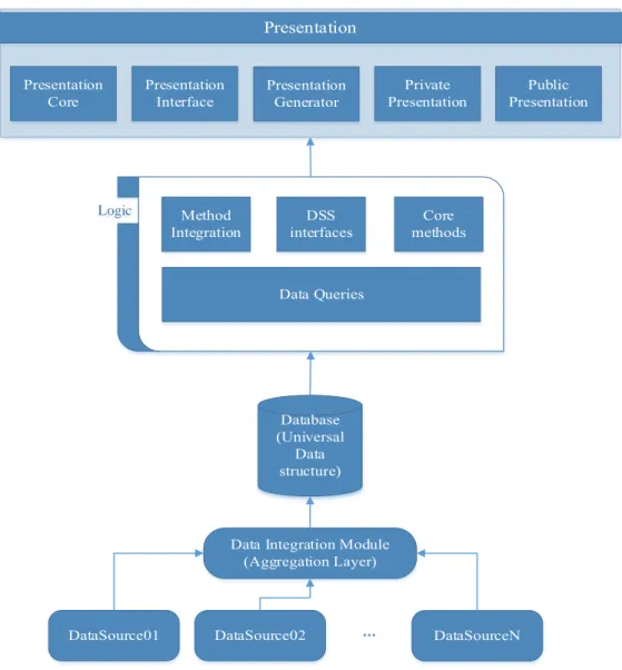
The overview of our UDSS is based on the three-layer architecture as it is summarized in Fig. 1.
Logic
...
Figure 1: Universal Decision Support System concept architecture
Definition. Universal Database structure (UDB) is a structure, which can receive and store any kinds of data, or at least there are trivial rules to transform original data formats to the universal database structure.
Definition. Data Integration Module (DIM) is a rule-based interface to define transformation rules to change original data structure into the UDB structure.
Definition. Data Queries (DQ) is a module executes queries to get the desired raw data from database.
Definition. Data Manipulation Module (DMM) is a set of algorithms, which can be performed to get scientific results, i.e., to support decision.
6
Definition. Core Methods (CM) contains algorithms, which are already in the system.
Definition. Method Integration (MI) supports the method integration process.
Definition. Decision Support System Interfaces give support to invoke algorithm implemented in another system.
Definition. Presentation Core (PC) is a set of views.
Definition. Presentation Generator (PG) supports the user to define presentation form based on entities of the performed algorithm.
Definition. Presentation Interfaces (PI) support the presentation subsystem integration process.
Definition. User Interface Module (UIM) helps the communication between the user and the system.
3.2. Validations and results
3.2.1. Use Case I: UDSS operation with current implementation
I examine how it is possible to implement decision support processes of the ForAndesT in my UDSS concept. ForAndesT is a decision support system in forestry. In forestry, there are couple of questions, which we would like to answer with a given DSS. These questions can be classified into the following types:
“What” question. Under the current circumstances (current land use type), what the land units’
performance will be. Land use type means tree species.
“What if” question. What the performance of a land unit would be, if initial land use type is converted into a new one, e.g., afforestation technique is changed replacing one tree species to another one.
“Where” question. Which land units are the best option under the user constrains.
I show an example for the “Where” question. The method behind answering this question is the Iterative Ideal Point Threshold (IIPT) developed by Annelies et al [50]. As the name of IIPT algorithm indicates, iterative search is performed based on Eq. 1.
𝑔𝑜𝑎𝑙_𝑣𝑎𝑙𝑢𝑒 = 𝑜𝑝𝑡𝑖𝑚𝑎𝑙_𝑣𝑎𝑙𝑢𝑒 ± 𝑖𝑡𝑒𝑟𝑎𝑡𝑖𝑜𝑛_𝑛𝑟 ∗ (max_𝑤𝑒𝑖𝑔ℎ𝑡
𝑤𝑒𝑖𝑔ℎ𝑡_𝐸𝑆 ) ∗ ( 𝑟𝑎𝑛𝑔𝑒
#𝑖𝑡𝑒𝑟𝑎𝑡𝑖𝑜𝑛), Eq. (1) where
optimal_value is minimum or maximum performance value according to the user definition;
iteration_nr is the number of iteration;
max_weight is the maximum weight among all selected attributes’ weights;
weight_ES is the weight of the given attribute;
range is the difference between the maximum and minimum value of the given attribute numeric co-domain;
#iteration is the actual iteration number.
7
The number of iterations is also defined by the user and this influences the number of sub-optimal solutions. Having performed IIPT, I get a sub-optimal answer. This answer shows which land units are suitable for the user defined performance attributes. It is rare that a land unit satisfying the preferences is found at the first run.
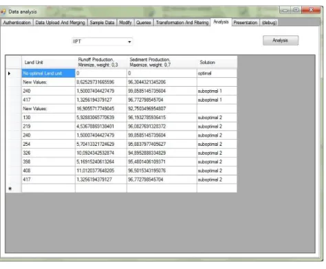
After performing the IIPT, the result is illustrated in Fig. 2.
Figure 2: IIPT result
In Fig. 2, we can see that there is no optimal land units, which satisfy the user defined conditions. However, there are sub-optimal ones. The UDSS concept offers the following solutions:
All data with proper uploading rules can be uploaded into the UDB.
If new data are measured, then it can be attached to the given main data row.
If I would like to use a new method, i.e., answer a new type of question, just the method itself must be created or called.
Data and methods can be combined easily.
Multi-criteria analysis can be performed on forestry data.
3.2.2. Use Case II: Ionogram processing
The UDSS helps not only existing forest decision support systems, but can be used in other fields like earth science, vendor selection, and production optimalization. UDSS was used to determine relevant area of the ionograms. Ionosphere’ layers are created by ionized gas with sunbeams. During the process, neutrons turn into positive or negative atom depending on they lose or receive an extra electron. The ionosphere can be divided into more layers. The lowest layer is D-layer, and going higher there are E-, F1- and F2- layers. The ionosphere measurement is made with the ionosonde. The data of ionosonde can be visualized as an ionogram, i.e., the ionosonde’s output is the ionogram. The ionogram is a binary picture, which contains a lot of noise and the relevant areas. The relevant areas have two main parts: (1) the ordinary
8
component and (2) the extraordinary component. An example of an ionogram is illustrated in Fig. 3, green is the ordinary and red is the extraordinary component. One of the challenges is to separate these two components from noises. The analysis of an ionogram has two main phases: (1) cleaning the data (filtering the noise from the picture) and (2) performing the desired analyzing techniques for the two components.
Another obstacle is the diversity of ionograms: general models cannot be defined. This is why the automatic processing of ionograms is not trivial. There are different partial solutions but none of them works in every ionogram.
Figure 4: Processed ionogram Figure 3: An ionogram example
9
In ionogram research, the curve of best fit is sought. The white curves are the best approximations of F1 and F2 in the example presented in Fig. 4. With the least squares approximation technique, the ionosphere consistency can be determined. This is the decision support part of the process. The approximations support to determine the right state of ionosphere at a given time. Ionogram components shape can be various, therefore it is possible that the curve of best fit is not found at the first time. For example, it is possible that not the fourth-degree equation makes the best result, but a fifth- or higher-degree fitting.
However, Sometimes the fitting algorithm does not work well on the specific ionogram due to its shape and further iterations are needed to get the results. If I use a filtering as a new DMM method in a new iteration, the result will be satisfying.
This example shows us how the UDSS can solve semi-structured problem. Using UDSS, the following advantage are:
Universal Database can also store ionogram data.
Original pictures are preserved, modification (analyzing) can be restored or saved.
All kinds of ionogram can be analyzed.
Several algorithms can be executed in each phase. (We used Connected-Component Labeling algorithm).
Both automatic and manual evaluation can be performed (semi-structured problem solving).
3.2.3. Use Case III: supplier performance analyzing
In the third case study, the optimization capability of UDSS is discussed. There is a wood production company where the color of the wooden material is the most important question, because the next production steps depend on it. Vendors ship boards to the company from the forest. Before the shipment, there are some preprocessing of the wood which are very crucial since some factor like drying time can has effect on the color of the wood. Therefore, the boards’ color is measured in the first step of the production line at this company.
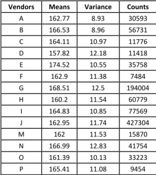
Table 1: Means and deviations of the vendors
Vendors Means Variance Counts
A 162.77 8.93 30593
B 166.53 8.96 56731
C 164.11 10.97 11776
D 157.82 12.18 11418
E 174.52 10.55 35758
F 162.9 11.38 7484
G 168.51 12.5 194004
H 160.2 11.54 60779
I 164.83 10.85 77569
J 162.95 11.74 427304
M 162 11.53 15870
N 166.99 12.83 41754
O 161.39 10.13 33223
P 165.41 11.08 9454
10
In this case, supplier, who better secures the pre-defined color of wood, has better performance.
Therefore that supplier will take better place on vendors’ ranking. The method of analysis is ANOVA. This method compares groups’ means, which allow me to determine whether the vendor performances differ or not. ANOVA has two conditions: (1) data items must follow the normal distribution and (2) variances must be homogeneous. Before applying ANOVA on the data, its conditions must be checked. The means and variances of the vendors are detailed in Table 1.
Based on Table 1, I can assume that variances are equal. But the properties of normality and homogeneity of variances must be proved. The classic normality chi test failed and I got the result value 2694.289 with the chi critical value 55.76 at level α = 0.05. The value is much bigger as the critical value, but I would expect to be lower based on the values of Table 1. I also checked normality with D’Agostino-Pearson Omnibus test, which analyzes the skewness and kurtosis and comes up with a single p-value.
Unfortunately, this test is failed as well. I used Bartlett-test to check homogeneity of variances. The result 15773.06 was much bigger than the critical value 59.334 at the same significance level.
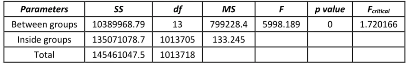
Table 2: ANOVA results
Parameters SS df MS F p value Fcritical
Between groups 10389968.79 13 799228.4 5998.189 0 1.720166
Inside groups 135071078.7 1013705 133.245
Total 145461047.5 1013718
There are related works where instead of these two prerequisites only the following condition is used:
ANOVA must be robust. Accepting this permissive condition, ANOVA can be performed and the result is summarized in Table 2.
In Table 2, the F value is much bigger than the critical value (α = 0.05). However, I can assume that the means are not regarded as equal (the smallest value is 157.82 and the biggest is 174.52 in Table 1), and ANOVA supports this theorem, but I can also see that F value is unduly big. To further investigate this interesting situation, Duncan test was applied. This test selects vendors, whose means are considered to be equal statistically. In other words, inside each groups generated by Duncan test, the means are regarded as equivalent statistically, i.e., if I execute ANOVA on each group selected by Duncan test, then the calculated F value will be lower than F critical value. However, no group was found, which means there are no means which are equal statistically according the Duncan test (α = 0.05). However, vendor F, J and M have nearly the same numerical values nearly in Table 1.
In this case study, the UDSS advantages were:
Vendor selection data can also be stored in UDSS.
Several algorithms can be performed.
Our data and analyzing process cannot be performed in ad-hoc DSS, however, vendor selection problem defined in another ad-hoc DSS can be solved using UDSS.
UDSS can solve optimalization problem as well.
UDSS can be used in company environment.
11
3.3. New results
Thesisgroup 1. I developed the concept for the Universal Decision Support System and showed it applications for three scientific problems originating from three different scientific fields.
Thesis 1.1 I proposed a new flexible universal database structure. Since the classic data warehouse structure does not support later modifications and its designation is mainly related to the business world, the suggested universal database can store any kind of data without modifications. The connections between data items, i.e., metadata and dimensions, are preserved.
Thesis 1.2 I designed the concept of the universal Data Integration Module which enables to gather information (data and metadata) from scattered data sources.
Thesis 1.3 I designed a generic Data Manipulation Module, which can store any kind of analyzing methods and a flexible Presentation Layer, which can be extended according to analysts’ design.
Thesis 1.4 Using three scenarios, I showed that the UDSS concept extends ad-hoc DSSs capabilities with unified data management, with analyzing model (filtering, transformation, and analyzing methods) independency and with presentation independency. Demonstrating the capabilities of the UDSS, we showed that a specified forestry decision problem, an automatic and semi-automatic ionogram processing problem and a vendor ranking problem can be solved in the same universal environment.
Related publications:
In English: [B1], [B3], [B6], [B7].
In Hungarian: [B2], [B4], [B5].
12
4. Random Correlation
Data are collected to analyze them and based on analysis results, decision alternatives are created. After making the decision, we act according to the selected decision, e.g., we define a correlation between two parameters based on the coefficient of determination or initiate production with the current settings of the new production machine. All decision processes have a validation phase, however, validation can generally only be done after the decision has been made. If we have made a false decision, then the consequences lead to a false correlation or to refuse materials. But how is it possible to make a wrong decision based on data and with precise mathematically proven analysis methods? My answer is a new theorem, which starts from the point that correlations between parameters and decision alternatives with following proper decision methodologies can be born randomly and this randomness is hidden also from analysts. Studying the state-of-the-art literature about statistical analyzes, I haven’t found any literature dealing with this phenomenon. So I started my work on the theory of Random Correlation.
4.1. Random Correlation Framework
4.1.1. Definition
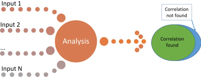
The main idea behind the random correlation is that data rows as variables present the revealed, methodologically correct results, however these variables are not truly connected, and this property is hidden from researchers as well. In other words, the random correlation theory states that there can be connection between data rows randomly which could be misidentified as a real connection with data analyses techniques.
There are lot of techniques to measure result’s endurance, such as r2, statistical critical values etc. I do not intent to replace these measurements with RC. The main difference between “endurance measurement”
values and RC is the approach of the false result. If we have a good endurance of the result, we strongly assume that the result is fair or the sought correlation exists. RC means that under the given circumstances (see Parameters Section), I can get results with good endurance. I can calculate r2 and critical values, I can make the decision based on them, but the result still can be affected by RC.
Figure 5: Sematic figure of Random Correlation
Analysis
Input 1 Input 2
...
Input N
Correlation found Correlation
not found
13
If we have the set of the possible inputs, the question is how the result can be calculated at all. In Fig. 5, it can be seen that in the set of results, the “correlation found” is highly possible, independent of which
“endurance measurement” method is performed.
4.1.2. Parameters
Every measured data has its own structure. Data items with various, but pre-defined form are inputs for the given analysis. I need to handle all kind of data inputs on the one hand, and to describe all analyzing influencing environment entities on the second hand. For example, if I would like to analyze a data set defined in UDSS with regression techniques, then I need the number of points, their x and y coordinates, the number of performed regressions (linear, quadratic, exponential) etc.
Having summarized, the random correlation framework parameters are:
k, which is the number of data columns;
n, which is the number of data rows;
r, which is the range of the possible numeric values;
t, which is the number of methods.
4.1.3. Models and methods
In the context of random correlation, there are two main models:
(1) We calculate the total possibility space (Ω-model);
(2) We determine the chance of getting a collision e.g., find a correlation (Θ-model).
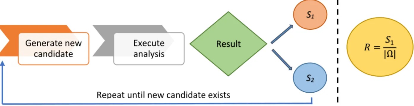
In the case of (1), all possible measurable combinations are produced. In other words, all possible n-tuples related to r(a,b) are calculated. Because of parameter r, I have a finite part of the number line, therefore this calculation can be performed. That is why r is necessary in our framework. All possible combinations must be produced, which the researchers can measure during the data collection. After producing all tuples, the method of analysis is performed for each tuple. If “correlated” judgment occurs for the given setup, then I increase the count of this “correlated” set S1 by 1. After performing all possible iterations, the rate R can be calculated by dividing S1 with |Ω|. R can be considered as a measurement of the “random occurring” possibility related to RC parameters. For example, if R is 0.99, “non-correlated” judgment can be observed only 1% of the possible combinations. The steps of Ω-model is summarized in Fig 6.
Figure 6: R calculation process
Generate new candidate
Execute
analysis Result
S1
S2
𝑅 = 𝑆1
|Ω|
Repeat until new candidate exists
14
In Fig. 6, S1 represents that correlation was found, while S2 represents that correlation has not been found.
In the case of (2), rate C is calculated. This shows how much data are needed to find a correlation with high possibility. Researchers usually have a hypothesis and then they are trying to proof their theory based on data. If one hypothesis is rejected, scientists try another one. In practice, we have a data row A and if this data row does not correlate with another, then more data rows are used to get some kind of connection related to A. The question is how many data rows are needed to find a certain correlation. I seek that number of data rows, after which correlation will be found with high possibility. This method is named Θ-model.
Based on value C, I have three possible judgements:
C is high. Based on the given RC parameters, it must be lots of dataset to get a correlation with high probability. This is the best result, because the chance of RC is low.
C is fair. The RC impact factor is medium.
C is low. The worst case. Relatively few datasets can produce good correlation.
4.1.4. Classes
RC can be occurred because of different causes. Data, the research environment, the methods of analysis can be different, therefore, classes are added to the framework. Each class is represented by a cause, which along the RC as phenomena can be appeared.
Class 1. Different methods can be applied for the given problem. If we cannot find good results with one method, then we choose another one. The number of analysis can be multiplied not just with the number of chosen methods but with methods’ different input parameters range and seeking and removing outliers. There could be some kind of error rate related to method’s results. It is not defined when the data are not related to each other. When we use more and more methods with different circumstances, e.g., different parameters and error rates, then we cannot be sure whether a true correlation was found or just a random one. If we increment the number of the methods, then there will be such a case when I surly find a correlation.
Class 2. Two (or more) methods produce opposite results. But this is not detected, since we stop at the first method with satisfying result. It is rather typical finding more precise parameters based on the
“correlation found” method. When methods are checked for this class, there can be two possibilities: (1) two or more methods give the same “correlated” result and (2) one or more methods do not present the same results. In option (1), we can assume that the data items are correlated truly with each other. In option (2), we cannot make a decision. It is possible, that the given methods present the inconsistent results occasionally or they always produce the conflict near the given parameters and/or data characteristics. There is a specific case in this group, when one method can be inconsistent with itself. It produces different type of results near given circumstances, e.g., sample size.
Class 3. The classic approach is that the more data we have, the more precise results we get. But it is a problem if a part of the data rows produces different results than the larger amount of the same data rows. For example, a data row is measured from start time t0 to time t, another is measured from start time t0 to time t + k, and the two data sets make inconsistent result. This is critical since we do not know which time interval we are in data collection. For this problem, the cross validation can be a solution. If all subsets of the data row for the time period t are not perform the same result, we only find a random model at high probability level. If they fulfill the “same result” condition, we find a true model likely.
15
This third group has another concept, which is slightly similar to the first one. We have huge amount of data sets in general, and we would like to get correlation between them. In other words, we define some parameters, which was or will be measured, and we analyze these data rows and create a model. We measure these data items further [time t + k]. If the new result is not the same as the previous one, we found a random model. The reason could be that a hidden parameter was missed from the given parameters list at the first step. It is possible, that the value of these hidden parameters change without our notice, and the model collapse. This kind of random correlation is hard to predict.
4.1.5. Candidates producing and simulation level
It is possible that Space Reducing Techniques (SRT) cannot grant enough space reduction in the case of huge RC parameter values. Therefore, simulation techniques must be applied to approximate the seeking of R.
Level 1. The trivial way to generate data rows randomly according to given k, n and r. I perform the analysis and notify the number of “correlated” and “non-correlated” cases. Based on these numbers, an R’ can be calculated. Based on the definition of possibility, R is approximated by R’. This is the fastest way to get an estimated R, however, calculating R’ would be precise only if the iteration i is large enough. After a certain level, performing i iterations cannot be possible in real time.
Level 2. The first phase of the SRT can be used to get more precise estimation of R. Because of the square function, the SRT first phase can be done quickly as I mention before. The problem is related to k, that is all k subsets must be produced from the result of the SRT first phase. However, if I produce all first phase candidates, i.e., use repeated permutation, and next, use simulation technique, i.e., randomly chosen k subsets in i iteration, then the second phase has an input, which contain only the accepted normal candidates. Therefore, more precise R’ can be determined.
Level 3. The first phase candidates preparation and the related frequency F can be combined. At Level 2, k data rows are chosen, but its weight is 1, i.e., one judgment is calculated. If a data row was chosen in an iteration, and since its F is known, I can define a weight based on this F. For example, in k = 3 case, at Level 2, just one judgment is, however, at Level 3, 𝐹1∗ 𝐹2∗ 𝐹3 judgments are produced. In other words, when three given data rows are selected, then as a matter of fact, all their permutations are chosen as well, because in the first phase, one row represents a combination with its own all permutations, i.e., frequency F. It is known that all Fk have the same result as in the case of Level 2. Therefore, I get more information in one iteration. In the next iteration, these 3 data rows [or neither their permutations of course] cannot be selected. This level produce more precise approximation of R with i iteration because of the known frequencies. The rate of Level 3 is signed with R*. R* approximates R better than R’. This level can be only use when the first phase can be calculated in real time.
4.2. ANOVA results related to Ω (R)
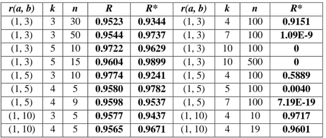
I calculate the whole possibility space and determine rate R for ANOVA. First, Space Reducing Technique (SRT) is used, the Level 2 simulation is applied. Table 3 has two main parts. In the first part, R and R* can be compared. The results show that approximation of R* is appropriate. To calculate R*, 1000 iterations were performed. In the second part, such cases are shown in which R cannot be calculated with self- developed Finding Unique Sequences (FUS) algorithm either. In these cases, only R* can be calculated in real time. First, the rates are high in the favor of H0. But in the case of large enough k and n, the rates are
16
heavily turn to H1. If the same experiment is performed with relatively small RC values, getting the result H0 and the “non-correlated” judgment is very high.
Table 3. ANOVA results using FUS and simulation
r(a, b) k n R R* r(a, b) k n R*
(1, 3) 3 30 0.9523 0.9344 (1, 3) 4 100 0.9151 (1, 3) 3 50 0.9544 0.9737 (1, 3) 7 100 1.09E-9 (1, 3) 5 10 0.9722 0.9629 (1, 3) 10 100 0 (1, 3) 5 15 0.9604 0.9899 (1, 3) 10 500 0 (1, 5) 3 10 0.9774 0.9241 (1, 5) 4 100 0.5889 (1, 5) 4 5 0.9580 0.9782 (1, 5) 5 100 0.0040 (1, 5) 4 9 0.9598 0.9537 (1, 5) 7 100 7.19E-19 (1, 10) 3 5 0.9577 0.9437 (1, 10) 4 10 0.9717 (1, 10) 4 5 0.9565 0.9671 (1, 10) 4 19 0.9601
Contrarily, the chance of H1 is increased with large enough values and “correlated” decision will be accepted at high possibility. However, this is a paradox in the view of big data inspired environment. In general, if we have a conclusion with smaller number of data items, then more data should enhance the conclusion. However, my results show that I can get contradictory results comparing cases with few data and big data inspired environment. By increasing k, the chance to find statistically equal data rows after each other in k-times can be “difficult”. In other words, increasing k, the chance to choose one data row (the kth) is high, which is not equal statistically with the other already chosen data rows (1, …, k-1).The answer can be proven by Θ-method. However, this answer does not affect the conclusion about the contradictory property of ANOVA.
4.3. Regression results related to Ω (R)
In this section, the regression techniques are described in the viewpoint of RC. Our standard analyzing steps are followed and noted in brackets. Regressions are in the first class of random correlation [Step 2].
If we have a set of data items and more and more regression techniques are used, then the chance of finding a correlation will be increased [Step 3]. Therefore, t is a critical parameter in this case [Step 4]. The k can be skipped, since I always have two columns, i.e., x and y coordinates, and therefore k = 2 is constant.
We have two parameter r: r1 determines the range of x values [r1(a1, b1)]), while r2 stands for range of the y values [r2(a2, b2)]). The count of the candidates is r1 ∗ r2 in the first phase. The calculation of Ω is based on k, n and r [Step 5]. The self-developed FUS can be used only partly: the first level of reduction cannot be applied since the order of the coordinates is important. For example, the x’ = {2, 1, 2} and y’ = {1, 3, 1}
do not give the same r2 as x = {1, 2, 2} and y = {1, 1, 3}. Therefore, all possibilities need to be directly produced in the first phase. However, the second level of reduction can be used without any modification.
We perform regression techniques and seek the best fitting line or curve. If I find high r2 with either of them, then I increase the count of “correlated” class, i.e. the number of 1’s. Oppositely, 0’s is increased by one. The acceptance level can be changed, I defined as r2 > 0.7. Also in regression case, the simulation deal with applying conditions. Assumptions must be checked in the case of regression techniques as well.
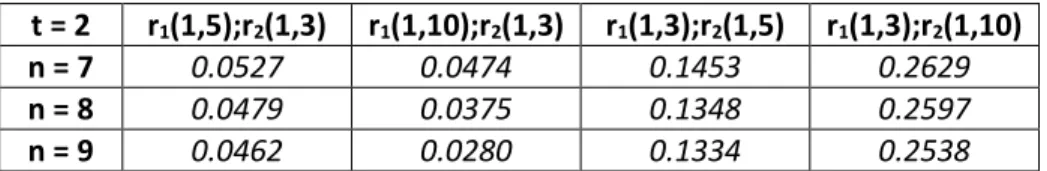
We can assume that independent property is satisfied. The normality is checked with D’Agostion-Pearson test. The homogeneity of variances is checked with Bartlett-test. Since I create all possible candidates, then X and Y can be seen as populations. The simulation can be run and R can be determined [Step 6]. I summarize the results in Table 4 when linear and exponential regressions were performed only, so t = 2.
17
Table 4. Results in the case of t = 2
t = 2 r1(1,5);r2(1,3) r1(1,10);r2(1,3) r1(1,3);r2(1,5) r1(1,3);r2(1,10)
n = 7 0.0527 0.0474 0.1453 0.2629
n = 8 0.0479 0.0375 0.1348 0.2597
n = 9 0.0462 0.0280 0.1334 0.2538
I increased n from 5 to 10, changed r1 and r2, used t = 4. The results are summarized in Table 5.
Table 5. Rates of r2 with t = 4
t = 4 r1(1,5);r2(1,3) r1(1,10);r2(1,3) r1(1,3);r2(1,5) r1(1,3);r2(1,10)
n = 5 0.2873 0.3071 0.3122 0.3288
n = 6 0.2092 0.2161 0.2530 0.3239
n = 7 0.1387 0.1379 0.2204 0.3102
n = 8 0.1142 0.1027 0.1947 0.3029
n = 9 0.1057 0.0796 0.1894 0.2927
By comparing Table 4 and 5, it can be concluded that the two extra methods increased the chance of r2 >
0.7, sometimes even doubled it. This means that it is possible to improve the rates by increasing t. The case of r1(1,3);r2(1,10) is very stable around 0.3. It is an important result, since the “correlated” and “non- correlated” judgments have the same chance in each cases. On the other side, it is rightful assumption, that the theoretically rate cannot be around 0.5 in regression case, because 0.5 would mean that the
“correlated” judgment is not more than a simple coin fifty-fifty rate. To say “correlated”, the rate must be stricter. Therefore, the parameters related to rate 0.3 could also be suitable. Further regression analyzing results are summarized in Table 6.
Table 6: Further regression results
r1(a1, b1); r2(a2, b2) n R (1, 3);(1, 3) 5 0.3465 (1, 3);(1, 3) 10 0.1087 (1, 5);(1, 5) 5 0.5332 (1, 5);(1, 5) 8 0.2491 (1, 5);(1, 5) 9 0.2196 (1, 4);(1, 6) 5 0.4153 (1, 4);(1, 6) 8 0.2406 (1, 4);(1, 6) 9 0.2248 (1, 6);(1, 4); 5 0.5419 (1, 6);(1, 4); 8 0.2472 (1, 6);(1, 4); 9 0.2147
If n is increased, the R decreases. If I assume further decreasing and observe the 30 sample rule of thumb, then the chance to get r2 > 0.7 is small. If we agree, that the connection between two variables must have smaller probability (not fifty-fifty), then regression techniques seems not be too sensitive to RC.
18
4.4. New results
Thesisgroup 2. To support the decision making process, I developed a framework named as Random Correlation. With the help of the framework, the results of the decision making process can be validated by several parameters to help the decisions.
Thesis 2.1 I defined the framework of Random Correlation to analyze methodologically correct results in which the variables are not truly connected. I defined four parameters and three classes, which can describe the environment to analyze random impact level.
Thesis 2.2 I defined two models: (1) the total possibility calculation and (2) the collision probability. The main though of the first one is to calculate all possible results and analyze the impact of randomness. The second one answers how many more data or analyzing methods must be used to get the desired “random”
result.
Thesis 2.3 I used the RC framework to analyze Analysis of Variance (ANOVA) statistical test to determine how big the random impact can be. I showed that ANOVA is very sensitive for random correlation at high possibility.
Thesis 2.4 I used the RC framework to analyze regression techniques to determine how big the random impact can be. I showed that regression techniques have a less random impact level.
Related publications:
In English: [B9], [B10], [B11]
In Hungarian: [B8]
19
References
[1] J. A. Khan, “Research methodology,” APH Publishing Corporation, New Delphi, 2008
[2] J. Kuada, “Research Methodology: A Project Guide for University Students,” Samfundslitteratur, Frederiksberg, 2012
[3] P. Lake, H. B. Benestad, B. R. Olsen, “Research Methodology in the Medical and Biological Sciences,” Academic Press, London, 2007
[4] A. Mohapatra, P. Mohapatra, “Research methodology,” Partridge Publishing, India, 2014
[5] G. D. Jackson, N.A. Moltschaniwskyj, "Spatial and temporal variation in growth rates and maturity in the Indo-Pacific squid Sepioteuthis lessoniana (Cephalopoda: Loliginidae)," Marine Biology, vol.
140, pp747−754, 2002
[6] G. T. Pecl, G. D. Jackson, “The potential impacts of climate change on inshore squid: biology, ecology and fisheries,” Reviews in Fish Biology and Fisheries, vol. 18, pp 373−385, 2008
[7] E. S. Zavaleta, B. D. Thomas, N. R. Chiariello, Gregory P. Asner, M. Rebecca Shaw, Christopher B.
Field, "Plants reverse warming effect on ecosystem water balance,” Proceedings of the National Academy of Sciences of the United States of America, vol. 100, pp9892–9893, 2003
[8] W. Liu, Z. Zhang, S. Wan, “Predominant role of water in regulating soil and microbial respiration and their responses to climate change in a semiarid grassland,” Global Change Biology, vol. 15, pp184–195, 2009
[9] J. A. Church, N. J. White, “A 20th century acceleration in global sea-level rise, “ Geophysical Research Letters, vol. 33, pp1−4, 2006
[10] J.R. Houston, R.G. Dean, “Sea-Level Acceleration Based on U.S. Tide Gauges and Extensions of Previous Global-Gauge Analyses,” Journal of Coastal Research, vol. 27, 409−417, 2011
[11] P. K. Aggarwal, R. K. Mall, “Climate Change and Rice Yields in Diverse Agro Environment of India.
II. Effect of Uncertainties in Scenarious and Crop Models on Impact assessment,” Climatic Change, vol. 52, pp331−343, 2002
[12] J. R. Welch, J. R. Vincent, M. Auffhammer, P. F. Moya, A. Dobermann, D. Dawe, “Rice yields in tropical/subtropical Asia exhibit large but opposing sensitivities to minimum and maximum temperatures,” Proceedings of the National Academy of Sciences of the United States of America, vol. 107, pp14562−14567, 2010
[13] L. Hooper, C. Bartlett, G. D. Smith, S. Ebrahim, “Systematic review of long term effects of advice to reduce dietary salt in adults,” British Medical Journal, vol. 325, pp628–632, 2002
[14] S. Pljesa, “The impact of Hypertension in Progression of Chronic Renal Failure,” Bantao Journal, vol. 1, pp71-75, 2003
[15] Climate Change 2007, Impacts, Adaptation, vulnerability, report, 2007
[16] H. Nkurunziza, J. Pilz, “Impact of increased temperature on malaria transmission in Burundi,”
International Journal of Global Warming, vol. 3, pp78−87, 2011
[17] P. Martens, R.S. Kovats, S. Nijhof, P. de Vries, M.T.J. Livermore, D.J. Bradley, J. Cox, A.J. McMichael,
“Climate change and future populations at risk of malaria,” Global Environmental Change, vol. 9, pp89−107, 1999
[18] P. W. Gething, D. L. Smith, A. P. Patil, A. J. Tatem, R. W. Snow, S. I. Hay, “Climate change and the global malaria recession,” Nature, vol. 465, pp342−345, 2010
[19] H. J. Fowlera, M. Ekstrom, “Multi-model ensemble estimates of climate change impacts on UK seasonal precipitation extremes,” International Journal of Climatology, vol. 29, pp385−416, 2009 [20] E. J. Burke, R. H. J. Perry, S. J. Brown, “An extreme value analysis of UK drought and projections of
change in the future,” Journal of Hydrology, vol. 388, pp131−143, 2010
20
[21] I. M. Held, T. L. Delworth, J. Lu, K. L. Findell, T. R. Knutson, “Simulation of Sahel drought in the 20th and 21st centuries,” Proceedings of the National Academy of Sciences of the United States of America, vol. 103, pp1152–1153, 2006
[22] R. J. Haarsma, F. M. Selten, S. L. Weber, M. Kliphuis, “Sahel rainfall variability and response to greenhouse warming,” Geophysical Research Letters, vol. 32, pp1−4, 2005
[23] A. Giannini, “Mechanisms of Climate Change in the Semiarid African Sahel: The Local View,”
Journal of Climate, vol. 23, pp743−756, 2010
[24] S. M. Crimmins, S. Z. Dobrowski, J. A. Greenberg, J. T. Abatzoglou, A. R. Mynsberge, “Changes in Climatic Water Balance Drive Downhill Shifts in Plant Species’ Optimum Elevations,” Science, vol.
331, pp324-327, 2011
[25] J. Grace, F. Berninger, L. Nagy, “Impacts of Climate Change on the Tree Line,” Annals of Botany, vol. 90, pp537−544, 2002
[26] T. A. Dueck, R. de Visser, H. Poorter, S. Persijn, A. Gorissen, W. de Visser, A. Schapendonk, J.
Verhagen, J. Snel, F. J. M. Harren, A. K. Y. Ngai, F. l. Verstappen, H. Bouwmeester, L. A. C. J.
Voesenek, A. van der Werf, “No evidence for substantial aerobic methane emission by terrestrial plants: a 13C-labelling approach,” New Phytologist, vol. 175, pp29−35, 2007
[27] F. Keppler, J. T. G. Hamilton, M. Braß, T. Röckmann, “Methane emissions from terrestrial plants under aerobic conditions,” Nature, vol. 439, pp187−191, 2006
[28] L. Siliang, L. Ronggao, L. Yang, “Spatial and temporal variation of global LAI during 1981–2006,”
Journal of Geographical Sciences, vol. 20, pp323−332, 2010
[29] G. P. Asner, J. M. O. Scurlock, J. A. Hicke, “Global synthesis of leaf area index observations:
implications for ecological and remote sensing studies,” Global Ecology and Biogeography, vol.
12, pp191−205, 2003
[30] C. Jaramillo, D. Ochoa, L. Contreras, M. Pagani, H. Carvajal-Ortiz, L. M. Pratt, S. Krishnan, A.
Cardona, M. Romero, L. Quiroz, G. Rodriguez, M. J. Rueda, F. de la Parra, S. Morón, W. Green, G.
Bayona, C. Montes, O. Quintero, R. Ramirez, G. Mora, S. Schouten, H. Bermudez, R. Navarrete, F.
Parra, M. Alvarán, J. Osorno, J. L. Crowley, V. Valencia, J. Vervoort, “Effects of Rapid Global Warming at the Paleocene-Eocene Boundary on Neotropical Vegetation,” Science, vol. 330, pp957−961, 2010
[31] L. F. Salazar, C. A. Nobre, M. D. Oyama, “Climate change consequences on the biome distribution in tropical South America,” Geophysical Research Letters, vol. 34, pp1−6, 2007
[32] M. Hulme, R. Doherty, T. Ngara, M. New, D. Lister, “African climate change: 1900–2100,” Climate Research, vol. 17, pp145−168, 2001
[33] A. P. Williams, C. Funk, “A westward extension of the warm pool leads to a westward extension of the Walker circulation, drying eastern Africa,” Climate Dynamics, vol. 37, pp2417−2435, 2011 [34] M.D. Flannigan, Y. Bergeron2, O. Engelmark, B.M. Wotton, “Future wildfire in circumboreal
forests in relation to global warming,” Journal of Vegetation Science, vol. 9, pp469−476, 1998 [35] E. S. Kasischke, N. L. Christensen, B. J. Stocks, “Fire, Global Warming, and the Carbon Balance of
Boreal Forests,” Ecological Applications, vol. 5, pp437−451, 1995
[36] M. E. Visser, A. C. Perdeck, J. H. Van Balen, C. Both, “Climate change leads to decreasing bird migration distances,” Global Change Biology, vol. 15, pp1859−1865, 2009
[37] N. Doswald, S. G. Willis, Y. C. Collingham, D. J. Pain, R. E. Green, B. Huntley, “Potential impacts of climatic change on the breeding and non-breeding ranges and migration distance of European Sylvia warblers,” Journal of Biogeography, vol. 36, pp1194−1208, 2009
[38] F. Pulido, P. Berthold, “Current selection for lower migratory activity will drive the evolution of residency in a migratory bird population,” Proceedings of the National Academy of Sciences of the United States of America, vol. 107, pp 7341−7346, 2010
21
[39] A. R. Huete, K. Didan, Y. E. Shimabukuro, P. Ratana, S. R. Saleska, L. R. Hutyra, W. Yang, R. R.
Nemani, R. Myneni, “Amazon rainforests green-up with sunlight in dry season,” Geophysical Research Letters, vol. 33, pp33−39, 2006
[40] A. Samanta, S. Ganguly, H. Hashimoto, S. Devadiga, E. Vermote, Y. Knyazikhin, R. R. Nemani, R. B.
Myneni, “Amazon forests did not green‐up during the 2005 drought,” Geophysical Research Letters, vol. 37, pp1−5, 2010
[41] D. T. Shindell, R. L. Miller, G. A. Schmidt, L. Pandolfo, “Simulation of recent northern winter climate trends by greenhouse-gas forcing,” Nature, vol. 399, pp452−455, 1999
[42] V. Petoukhov, V. A. Semenov, “A link between reduced Barents-Kara sea ice and cold winter extremes over northern continents,” Journal of Geophysical Research, vol. 115, D21111, 2010 [43] P. Knippertz, U. Ulbrich, P. Speth, “Changing cyclones and surface wind speeds over the North
Atlantic and Europe in a transient GHG experiment,” Climate Research, vol. 15, pp109−122, 2000 [44] R. Vautard, J. Cattiaux, P. Yiou, J.-N. Thépaut, P. Ciais, “Northern Hemisphere atmospheric stilling partly attributed to an increase in surface roughness,” Nature Geoscience, vol. 3, pp756−761, 2010
[45] I. Bogardi, I. Matyasovzky, “Estimating daily wind speed under climate change,” Solar Energy, vol.
57, pp239−248, 1996
[46] M. Rebetez, R. Lugon, P.-A. Baeriswyl, “Climatic Change and Debris Flows in High Mountain Regions: The Case Study of the Ritigraben Torrent (Swiss Alps),” Climatic Change, vol. 36, pp371−389, 1997
[47] M. Stoffel, M. Beniston, “On the incidence of debris flows from the early Little Ice Age to a future greenhouse climate: A case study from the Swiss Alps,” Geophysical Research Letters, vol. 33, L16404, 2006
[48] M. Stoffel, M. Bollschweiler, M. Beniston, “Rainfall characteristics for periglacial debris flows in the Swiss Alps: past incidences–potential future evolutions,” Climatic Change, vol. 105, pp263−280, 2011
[49] B. Nosek et al. (Open Science Collaboration),“Estimating the reproducibility of psychological science,” Science, vol. 28, aac4716, 2015
[50] A. De Meyer, R. Estrella, P. Jacxsens, J. Deckers, A. Van Rompaey, J. Van Orshoven, “A conceptual framework and its software implementation to generate spatial decision support systems for land use planning,” Land Use Policy, vol. 35, pp.271–282, 2013
22
List of Publications
Universal Decision Support System
[B1] Jos M.F. Van Orshoven, Vincent Kint, Anja Wijffels, René Estrella, Gergely Bencsik, Pablo Vanegas, Bart Muys, Dirk Cattrysse, Stefaan Dondeyne, “Upgrading Geographic Information Systems to Spatio- Temporal Decision Support Systems”, Mathematical and Computational Forestry & Natural-Resource Sciences, vol. 3, pp36−41, 2011
[B2] Gergely Bencsik, Attila Gludovátz, László Jereb, “Integrált informatikai elemző keretrendszer alkalmazása a magyar felsőoktatásban”, Proc. of Informatika a felsőoktatásban konferencia 2011, pp1040−1047, Debrecen, Hungary, 2011 (In Hungarian)
[B3] Gergely Bencsik, Attila Gludovátz, László Jereb, “Adaptation of analysis framework to industry related economic problems”, Proc. of The Impact of Urbanization, Industrial and Agricultural Technologies on the Natural Environment: International Scientific Conference on Sustainable Development and Ecological Footprint, pp1−6, Sopron, Hungary, 2012
[B4] Gergely Bencsik, Attila Gludovátz, “Univerzális elemző keretrendszer gazdasági alkalmazásának lehetőségei különös tekintettel a termelővállalatokra”, Proc. of International Symposium on Business Information Systems (OGIK 2012), pp36−37, Győr, Hungary, 2012 (In Hungarian)
[B5] Gergely Bencsik, Attila Gludovátz, László Jereb, “Decision support framework with wood industrial application”, Proc. of 8th International PhD & DLA Symposium, pp154, Pécs, Hungary, 2012
[B6] Gergely Bencsik, Attila Gludovátz, “Adaptation of a universal decision support system in forestry”, Proc. of Implementation of DSS tools into the forestry practice, Technical University Zvolen, pp37−49, 2013 [B7] Gergely Bencsik, László Bacsárdi, “Towards to decision support generalization: the Universal Decision Support System Concept”, Proc. of IEEE 19th International Conference on Intelligent Engineering Systems (INES), pp277−282, Bratislava, Slovakia 2015
Random Correlation
[B8] Gergely Bencsik, László Bacsárdi, “Statisztikai adatok közötti véletlen összefüggések tanulmányozása”, Proc. of Informatika a felsőoktatásban konferencia 2014, pp403−412, Debrecen, Hungary, 2014 (In Hungarian)
[B9] Gergely Bencsik, László Bacsárdi ,“Effects of Random Correlation on ANOVA and Regression”, Proc.
of the 9th International Conference on Knowledge, Information and Creativity Support Systems, pp396−401, Lemesos, Cyprus, 2014
[B10] Gergely Bencsik, László Bacsárdi, “New Methodology to Analyze the Random Impact Level of Mathematically Proved Results”, Proc. of 15th IEEE International Symposium on Computational Intelligence and Informatics (CINTI), pp33−38, Budapest, Hungary, 2014
23
[B11] Gergely Bencsik, László Bacsárdi, “Novel methods for analyzing random effects on ANOVA and regression techniques”, (to be published in Springer Advances in Intelligent Systems and Computing, ISSN 2194-5357)
Other publications
[B12] Attila Gludovátz, Gergely Bencsik, “Egy felsőoktatási képzés Balanced Scorecard alapú mintarendszer működésének demonstrálása”, Proc. of 5th International Symposium on Business Information Systems, pp88, Győr, Hungary, 2007 (In Hungarian)
[B13] Gergely Bencsik, Attila Gludovátz, László Bacsárdi, “Tudásmenedzsment módszerek faipari alkalmazása”, Proc. of. Inno Lignum konferencia, Sopron, Hungary, 2010 (In Hungarian)
[B14] Gergely Bencsik, “Analyzing the Adaptability Condition of Decision Support Systems and Data mining in Forestry”, Short Time Scientific Mission report, COST FP0804, Leuven, Belgium, 2010
[B15] Márton Edelényi, Gergely Bencsik, Attila Gludovátz, “Adaptation possibilities of knowledge management tools in higher education”, Proc. of. Szellemi tőke, mint versenyelőny avagy A tudásmenedzsment szerepe a versenyképességben, pp883−897, Komárno, Slovakia, 2010
[B16] Gergely Bencsik, Attila Gludovátz, “Experience with universal data analyses”, Proc. of Forest Management Decision Support Systems (FORSYS) Conference, COSTFP0804, pp53−54, Umea, Sweden, 2013
[B17] Gergely Bencsik, “Virtual Environment to simulate business processes related to ERP systems”, Presentation on Microsoft Dynamics Convergence 2014 conference, Barcelona, Spain, 2014
[B18] Gergely Pieler, Gergely Bencsik, “Relevant and related area extraction from binary images”, Proc.
of 11th International Symposium on Business Information Systems, Budapest, Hungary, 2014
[B19] Péter Kiss, Gergely Bencsik, “Virtual Economic Environment”, Proc. of 11th International Symposium on Business Information Systems, Budapest, Hungary, 2014
[B20] Péter Kiss, Gergely Bencsik, László Bacsárdi, “From ERP trainings to business: a new approach of simulations in economics”, Proc. of 12th International Symposium on Business Information Systems, pp49−50, Veszprém, Hungary, 2015
[B21] Attila Gludovátz, Gergely Bencsik, László Bacsárdi, “IT challenges of a production system”, Proc. of 12th International Symposium on Business Information Systems, pp31, Veszprém, Hungary, 2015