New Approach to Fuzzy Decision Matrices
Pavla Rotterová, Ondřej Pavlačka
Department of Mathematical Analysis and Applications of Mathematics, Faculty of Science, Palacký University Olomouc, 17. listopadu 1192/12, 771 46 Olomouc, Czech Republic, pavla.rotterova01@upol.cz, ondrej.pavlacka@upol.cz
Abstract: Decision matrices represent a common tool for modeling decision-making problems under risk. They describe how the decision-maker's evaluations of the considered alternatives depend on the fact which of the possible and mutually disjoint states of the world will occur. The probabilities of the states of the world are assumed to be known. The alternatives are usually compared on the basis of the expected values and the variances of their evaluations. However, the states of the world as well as the alternatives evaluations are often described only vaguely. Therefore, we consider the following problem: the states of the world are modeled by fuzzy sets defined on the universal set on which the probability distribution is given, and the evaluations of the alternatives are expressed by fuzzy numbers. We show that the common approach to this problem, based on employing crisp probabilities of the fuzzy states of the world computed by the formula proposed by Zadeh, is not appropriate. Therefore, we introduce a new approach in which a fuzzy decision matrix does not describe discrete random variables but fuzzy rule bases. The problem is illustrated by an example.
Keywords: decision matrices; fuzzy decision matrices; decision making under risk; fuzzy states of the world; fuzzy rule bases system
1 Introduction
A decision matrix is often used as a tool of risk analysis in decision making under risk [3], [4], [7], [14]. It describes how the decision-maker's evaluations of the considered alternatives depend on the fact which of the possible and mutually disjoint states of the world will occur. The probabilities of occurrences of these states of the world are supposed to be known. Thus, the evaluations of the alternatives are discrete random variables. The alternatives are usually compared on the basis of the expected values and the variances of their evaluations. The decision-maker selects the alternative that maximizes his/her expected evaluation or maximizes the expected evaluation and simultaneously minimizes the variance.
In practical applications, the states of the world as well as the evaluations of the alternatives can be determined vaguely. The states of the world are mostly
described verbally, like "the gross domestic product will increase moderately during next year". Sometimes, it can be problematic to express the evaluations of alternatives precisely because we may not have enough information. For instance, the evaluation under a certain state of the world can be described as “about 5%”.
In some cases, it is more natural for a decision-maker to express the evaluations by selecting a term from a given linguistic scale.
The vaguely described pieces of information can be mathematically modeled by means of tools of fuzzy sets theory. Different views of uncertainty and fuzzy decisions in a decision matrix are discussed in [7]. Multiple attribute decision making problems, described by a decision matrix with crisp and fuzzy data, are analyzed in [1]. In [2], a fuzzy decision matrix is applied to a group decision making. An application of risk analysis with fuzzy sets employing the decision matrix is presented in [3]. In [4], the authors considered decision matrices with fuzzy targets. In [5], the hesitant fuzzy decision matrix, i.e. a decision matrix containing fuzzy sets with a different definition of membership function then the original one proposed by Zadeh [15], is considered.
A decision matrix with the fuzzy states of the world and the fuzzy evaluations of the alternatives under the particular fuzzy states of the world is called a fuzzy decision matrix. In [Error! Reference source not found.2], the authors considered a model where the fuzzy states of the world are expressed by fuzzy sets on the universal set on which the probability distribution is given. They proposed to proceed in the same way as in the case of the crisp (i.e. exactly described) states of the world; they set the probabilities of the fuzzy states of the world applying the formula proposed by Zadeh in [17]. Within this approach, the evaluations of the alternatives are understood as discrete random variables taking on fuzzy values with the probabilities of the fuzzy states of the world.
In [10], the authors showed that the Zadeh’s probabilities of fuzzy events lack the common interpretation of a probability measure. Another problem is a precise definition of "the occurrence of the particular fuzzy state of the world" (see the discussion in Section 3.3). Therefore, an alternative to how the information contained in a fuzzy decision matrix can be treated was proposed in [8]. The way is based on the idea that a fuzzy decision matrix does not determine discrete fuzzy random variables, but a system of fuzzy rule bases (a fuzzy rule base was introduced in [16]). However, only the crisp (i.e. not fuzzy) evaluations of alternatives were considered in [8] which makes the problem much simpler. The main aim of the paper is to extend this approach to the case where the evaluations of alternatives are expressed by fuzzy numbers, and to derive the formulas for correct computations of fuzzy expected values and fuzzy variances of evaluations of alternatives. The obtained fuzzy characterstics will be compared with those obtained by the approach considerd in [12].
The paper is organized as follows. A decision matrix tool is briefly recalled in Section 2. In Section 3, the common approach to the fuzzification of a decision
matrix is analysed and the related problems are discussed. Our new approach to this problem is introduced and analysed in Section 4. In Section 5, both approaches are compared by an illustrative example.
2 Decision Matrices
In this section, let us describe a decision matrix as a tool for supporting a decision making under risk.
Let us consider a probability space (Ω, 𝒜, P) where Ω denotes a non-empty universal set of all elementary events, 𝒜 is a σ-algebra of subsets of Ω, i.e. 𝒜 represents the set of all considered random events, and P: 𝒜 → [0,1] denotes a probability measure.
Now, let us describe a decision matrix under risk, considered e.g. in [3], [4], [7]
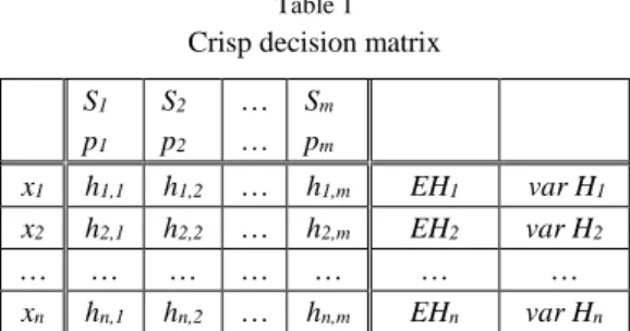
and [14]. The decision matrix is shown in Table 1. In the matrix, x1, x2, …, xn
represent the alternatives of a decision-maker, S1, S2, …, Sm, where Sj ∈ 𝒜 for j = 1, 2, …, m, denote the mutually disjoint states of the world, i.e. Sj ∩ Sk = ∅ for any j, k ∈ {1, 2, …, m}, j ≠ k, and mj1SjΩ, p1, p2, …, pm stand for the probabilities of the states of the world S1, S2, …, Sm, i.e. pj = P(Sj), and for any i ∈ {1, 2, …, n} and j ∈ {1, 2, …, m}, hi,j means the decision-maker's evaluation if he/she chooses the alternative xi and the state of the world Sj occurs. The evaluation of the alternative xi is commonly understood as a discrete random variable Hi: {S1, S2, …, Sm} → ℝ which takes on the values hi,j = Hi(Sj) with the probabilities pj, j = 1, 2, …, m.
Table 1 Crisp decision matrix S1
p1
S2
p2
…
… Sm
pm
x1 h1,1 h1,2 … h1,m EH1 var H1
x2 h2,1 h2,2 … h2,m EH2 var H2
… … … … …
xn hn,1 hn,2 … hn,m EHn var Hn
The alternatives are usually compared on the basis of the expected values and the variances of their evaluations (an overview of decision making rules can be found e.g. in [Error! Reference source not found.]). The expected values of the decision-maker's evaluations, denoted by EH1, EH2, …, EHn, are given for any i ∈ {1, 2, …, n} by:
m
j=
i,j j
i
= p h .
EH
1
(1)
The variances of the decision-maker's evaluations, denoted by var H1, var H2, …, var Hn, are calculated for any i ∈ {1, 2, …, n} as follows:
m
j=
i i,j j
i
= p h EH .
var H
1
)
2(
(2)The alternative that maximizes the expected evaluation and minimizes the variance of the evaluation is selected as the best one.
3 Fuzzy Decision Matrices
Now, let us describe the common approach to the generalization of a decision matrix to the case where the states of the world and the evaluations of the alternatives are expressed by fuzzy sets, considered e.g. in [Error! Reference source not found.2]. Within this approach, the probabilities of the fuzzy states of the world, computed by the formula proposed by Zadeh in [17], are used for computations of the characteristics of the evaluations of the alternatives.
3.1 Fuzzy States of the World
Vaguely defined states of the world can be mathematically expressed by fuzzy sets. A fuzzy set A on a non-empty set Ω is determined by its membership function μA: Ω → [0, 1]. Let us denote the family of all fuzzy sets on Ω by ℱ(Ω).
A support of A and a core of A are given as SuppA:=
ωΩ|μA(ω)>0
and CoreA:=
ωΩ|μA(ω)1
, respectively. Aα means an α-cut of A, i.e. )
: = ω Ω | μ (ω
A
α A for any α ∈ (0,1].Remark Any crisp set A ⊆ Ω can be seen as a fuzzy set A ∈ ℱ(Ω) of a special kind where its characteristic function χA coincides with the membership function μA of the fuzzy set. In fuzzy models, this convention allows us to consider also precisely described events given by crisp sets.
In fuzzy decision matrices, fuzzy states of the world are described by the fuzzy events. According to Zadeh [17], a fuzzy event A ∈ ℱ (Ω) is a fuzzy set whose α - cuts are random events, i.e. Aα ∈ 𝒜 for all α ∈ (0,1]. As an analogy to a decomposition of the universal set Ω by crisp states of the world, the fuzzy states of the world, denoted by S1, S2, …, Sm, have to form a fuzzy partition of the universal set Ω, i.e. for any ω ∈ Ω, it has to hold that
m
j Sj 1
.
1
(3)Zadeh [17] extended the crisp probability measure P to the case of fuzzy events.
Let us denote this extended measure by PZ. A probability PZ (A) of a fuzzy event A is defined as follows:
A : = E μ =
μ ω dP .
P
Z A A (4)3.2 Fuzzy Evaluations of Alternatives under the Particular Fuzzy States of the World
As was mentioned in Introduction, it can be difficult for a decision-maker to evaluate each alternative under each state of the world by a real number. One reason can be a lack of information caused e.g. by inaccuracies of measurements or a lower quality of data transmissions. Another reason can be that it is more natural for the decision-maker to describe the evaluations linguistically rather than by numbers.
Linguistic terms or uncertain quantities can be mathematically modeled by fuzzy numbers. A fuzzy number A is a fuzzy set on the set of all real numbers ℝ such that its core A is non-empty, its α-cuts Aα are closed intervals for any α ∈ (0, 1], and its support Supp A is bounded. The family of all fuzzy numbers on ℝ will be denoted by ℱN(ℝ). In some models, fuzzy evaluations can be restricted only to a closed interval, mostly [0,1]. A fuzzy number defined on the interval [a, b] is a fuzzy number whose α-cuts belong to the interval [a, b] for all α ∈ (0,1].
The family of all fuzzy numbers on the interval [a, b] will be denoted by ℱN([a, b]).
Thus, there are two ways of expressing a fuzzy evaluation of an alternative. The first way is to specify the evaluation directly by a fuzzy number. For instance, some expert can evaluate the particular alternative directly by the fuzzy number
"about five percent profit", whose membership function is shown in Figure 1.
The second possibility of expressing the fuzzy evaluation of the alternative consists in the fact that the evaluation is modeled by a linguistic variable (linguistic variables were introduced in [16]). A decision-maker evaluates the alternatives under the particular states of the world by appropriate linguistic terms whose mathematical meanings are described by fuzzy numbers. A set of linguistic terms 𝒯1, 𝒯 2, …, 𝒯r forms a linguistic scale on [a, b] if T1, T2, …, Tr ∈ ℱN([a, b]) representing their mathematical meanings form a fuzzy partition of [a, b].
Figure 1
Example of an expertly specified evaluation
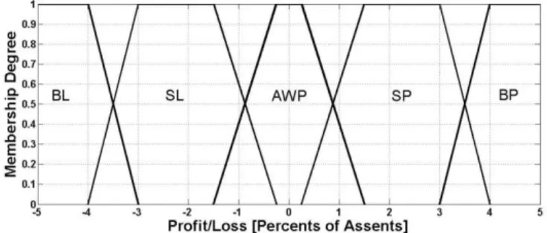
Example Let us consider a linguistic scale shown in Figure 2. This scale is formed by the linguistic terms "a big loss" (BL), "a small loss" (SL),
"approximately without profit" (AWP), "a small profit" (SP), and "a big profit"
(BP). In some cases, a selection of some linguistically described value like
"a small profit" from the given linguistic scale can be more convenient for a decision-maker.
Figure 2 Example of a linguistic scale
3.3 Common Approach to a Fuzzy Decision Matrix
Let us describe a common approach to a fuzzy decision matrix that was considered e.g. in [Error! Reference source not found.2].
In the fuzzy decision matrix given in Table 2, x1, x2, …, xn denote the alternatives of the decision-maker and S1, S2, …, Sm stand for the fuzzy states of the world.
Probabilities of the fuzzy states of the world S1, S2, …, Sm, calculated according to (4), are denoted by pZ1, pZ2, …, pZm, i.e. pZj = PZ(Sj). For any i ∈ {1, 2, …, n} and j ∈ {1, 2, …, m}, Hi,j expresses the fuzzy evaluation of the alternative xi under the fuzzy state of the world Sj.
Table 2 Fuzzy decision matrix S1
pZ1
S2
pZ2
…
… Sm
pZm
x1 H1,1 H1,2 … H1,m EH1Z var H1Z
x2 H2,1 H2,2 … H2,m EH2Z var H2Z
… … … …
xn Hn,1 Hn,2 … Hn,m EHnZ var Hn Z
Thus, the evaluation of the alternative xi is understood as a discrete fuzzy random variable HiZ: {S1, S2, …, Sm} → ℱN(ℝ) where HiZ(Sj) = Hi,j for j=1, 2, …, m. Its fuzzy expected value, denoted by EHiZ, is computed according to the generalized formula (1) where the probabilities pj of the states of the world are replaced by the Zadeh's probabilities pZj of the fuzzy states of the world and the crisp evaluations hi,j are replaced by the fuzzy evaluations Hi,j, i.e.
.
1
m
j=
j i, Zj Z
i
= p H
EH
(5)The α-cuts
iZUα
ZL α i Z
i,α= Eh ,Eh
EH , , are obtained for all α ∈ (0,1] as follows: Let
i,j,αU
L i,j,α
i,j,α h h
H , , j = 1, 2, …, m. The boundary values of
EH
i,αZ are obtained by
m
j=
L α j i, Zj ZL
i,α
= p h
Eh
1
, (6)
and
m
j=
U α j i, Zj ZU
i,α
= p h
Eh
1
,
.
(7)Computation of the fuzzy variance var HiZ is more complex. It was shown in [9]
that the formulas proposed in [Error! Reference source not found.2] were not correct because the relationships between the fuzzy evaluations Hi,1, Hi,2,…, Hi,m, and the fuzzy expected evaluation EHiZ were not involved in the calculation. This fact causes that the uncertainty of the resulting fuzzy variance is falsely increased.
The proper formulas for the computation of the fuzzy variance were proposed in [9]. For any i ∈ {1, 2, ..., n} and any α ∈ (0,1], the α-cut of the fuzzy variance
i,αZU
ZL i,α Z
i,α= var h var h
var H , has to be calculated as follows: Let us denote
m
j=
m
= k
k i, Zk j
i, Zj m
i i i
i
h h h = p h p h
1
2
1 ,
2 , 1
,
, , ..., .
z
(8)Then,
h h h | h H , j = , m
=
var h
i,αZLmin z
i i,1,
i,2, ...,
i,m i,j
i,j,α1,2,...
(9) and
h h h | h H , j = , m
var h
i,αZU max z
i i,1,
i,2, ...,
i,m i,j
i,j,α1,2,...
. (10) As it is written in section 2, the element hi,j of the matrix given in table 1 describes the decision-maker's evaluation of the alternative xi if the state of the world Sjoccurs. If we consider the fuzzy states of the world instead of the crisp ones, a natural question arises: What does it mean to say "if the fuzzy state of the world Sj
occurs"? Let us suppose that some ω ∈ Ω has occurred. If μ
=1,Sj
then it is clear that the evaluation of the alternative xi is exactly hi,j. However, what is the evaluation of xi if 0
1Sj
μ (which also means that 0
1Sk
μ for some
k ≠ j)? Thus, perhaps it is not appropriate in the case of a decision matrix with the fuzzy states of the world to treat the evaluation of xi as a discrete random variable HiZ that takes on the fuzzy values Hi,1, Hi,2,…, Hi,m.
Moreover, it was pointed out by Rotterová and Pavlačka [10] that the Zadeh’s probabilities pZ1, pZ2, …, pZm of the fuzzy states of the world express the expected membership degrees in which the particular states of the world will occur. Thus, they do not have in general the common probabilistic interpretation - a measure of a chance that a given event will occur in the future, which is desirable in the case of a decision matrix.
Therefore, we cannot say that the values EH1Z, EH2Z, ..., EHnZ, given by (6) and (7), and var H1Z, var H2Z, ..., var HnZ, given by (9) and (10), express the expected values and variances of evaluations of the alternatives, respectively. Ordering of the alternatives based on these characteristics is questionable.
4 Fuzzy Rule Bases System Determined by the Fuzzy Decision Matrix
In this section, let us introduce a different approach to the model of decision making under risk described by the decision matrix with fuzzy states of the world presented in Table 2. Taking the problems discussed in the previous section into account, we suggest not to treat the evaluation of the ith alternative xi, i ∈ {1, 2, …, n}, as a discrete random variable HiZ taking on the fuzzy values Hi,1, Hi,2, ..., Hi,m
with the probabilities pZ1, pZ2, …, pZm. Instead of this, we propose to understand the information about the evaluation of the alternative xi as the following fuzzy rule base:
If the state of the world is S1, then the evaluation of xi is Hi,1. If the state of the world is S2, then the evaluation of xi is Hi,2.
⋮ (11)
If the state of the world is Sm, then the evaluation of xi is Hi,m.
In [8], it was shown that in the case of the fuzzy decision matrix with crisp evaluations under the particular fuzzy states of the world, it is appropriate to use the Sugeno’s method of fuzzy inference, introduced in [11]. The obtained output from the fuzzy rule base was expressed by a real number.
In the paper, we deal with the fuzzy evaluations of the alternatives under the fuzzy states of the world. Thus, the so-called generalised Sugeno’s method of fuzzy inference, introduced in [13], should be applied for obtaining an output from the fuzzy rule base (11). According to this method, the evaluation of an alternative xi for a given ω ∈ Ω is computed in the following way:
m= j
j j i,
m S
=
j Sj
m
= j
j j i,
S S
i
= μ ω H
ω μ
ω H μ ω =
H
1 1
1
.
(12)For any α ∈ (0,1], let us denote
i,Ujα
L jα α i, j
i
= h h
H
,, ,,
, , j = 1, 2, …, m, and
iSUα
SL α i S
α
i = h h
H, , , , . Then, the boundary values of HiS,α
are computed as follows:
m
j=
L α j j i,
S SL
α
i
ω = μ ω h
h
1
, ,
and
m
j=
U α j j i,
S SU
α
i
ω = μ ω h
h
1
,
,
.
Remark In the formula (12), the denominator equals to one due to the assumption that the fuzzy states of the world S1, S2, …, Sm form a fuzzy partition of Ω. It is worth to note that in our approach, this assumption can be omitted.
Since we operate within the given probability space (Ω, 𝒜, P), HiS is a fuzzy random variable such that HiS: Ω → ℱN(ℝ).
Remark It can be easily seen from (12) that in the case of the crisp states of the world Sj, j = 1, 2, …, m, and the crisp evaluations hi,j, i = 1, 2, …, n, under the particular fuzzy states of the world, the fuzzy random variables HiS coincide with discrete random variables Hi taking on the values hi,j with the probabilities pj,
j = 1, 2, …, m. Thus, this new approach can be seen as an extension of a decision matrix to the case of the fuzzy states of the world and the fuzzy evaluations of alternatives where appropriate.
Analogously, as in the common approach to the fuzzy decision matrix, the ordering of the alternatives x1, x2, …, xn can be based on the fuzzy expected values and the fuzzy variances of the random variables HiS, i = 1, 2, …, n. Let us introduce the formulas for computations of the α-cuts of EHiS and var HiS.
For any α ∈ (0,1], the α-cut of the fuzzy expected output from the fuzzy rule base given by (11), denoted by ,
, , ,
,SU α i SL
α i S
α
i = Eh Eh
EH is obtained as follows:
ω h dP μ
m ,
= j , H h dP ω h
μ
= Eh
m
= j
L α j i, S
α j
i, m
= j
j i, S
SL α i
j
j
1
,
j, i, 1
,
min 1,2,...
(13)
and
.
1,2,...
max
1
,
j, i, 1
,
dP ω h
μ
m ,
= j , H h dP ω h
μ
= Eh
m
j=
U α j i, S
α j
i, m
j=
j i, S
SU α i
j
j
(14)
The α-cut
i,αSU
SL i,α S
i,α= var h var h
var H , of the fuzzy variance of the output from the fuzzy rule base is obtained as follows: Let us denote
. )
..., , , s
2
1 1
, 2 , 1 ,
dP dP h μ (t) h
μ (ω
=
h h h
m
j t
m
k
k k i, S j
j i, S
m i i i i
(15)
Then,
h h h | h H , j = , m
=
var h
i,αSLmin s
i i,1,
i,2, ...,
i,m i,j
i,j,α1,2,...
(16) and
h h h | h H , j = , m
=
var h
i,αSUmax s
i i,1,
i,2, ...,
i,m i,j
i,j,α1,2,...
. (17) Now, let us compare the fuzzy expected values EHiZ and EHiS, and the fuzzy variances var HiZ and var HiS.Theorem 1 For i = 1, 2, …, n, the expected fuzzy evaluation EHiZ and the expected output from the fuzzy rule base EHiS coincide.
Proof For any α ∈ (0,1], let
iSUα
SL α i S
α
i = Eh Eh
EH, , , , be the α-cut of the expected output from the fuzzy rule base and
iZUα
ZL α i Z
α
i = Eh Eh
EH, , , , be the α-cut
of the fuzzy expected evaluation. For the boundary values of
EH
iS,α, it holds:
ZL α i L
α j i, m
j=
Zj
m
j=
L α j j i,
S m
j=
L α j j i,
S SL
α i
Eh
= h p
h ω dP μ
= dP ω h
μ
= Eh
, ,
1
1
, 1
, ,
and
,
.
, 1
1
, 1
, ,
ZU α i U
α j i, m
j=
Zj
m
j=
U α j j i,
S m
j=
U α j j i,
S SU
α i
Eh
= h p
h ω dP μ
= dP ω h
μ
= Eh
Thus, all the α-cuts are the same. Therefore, EHiS = EHiZ. □ In [8], the authors showed that in the case of a fuzzy decision matrix where the evaluations under the particular fuzzy states of the world are expressed by real numbers, the variances var HiZ and var HiS are real numbers as well, and var HiZ
≥ var HiS. Now, let us compare the fuzzy variances var HiZ and var HiS.
Theorem 2 For i = 1, 2, …, n, the fuzzy variance var HiZ of the fuzzy evaluation is greater or equals to the fuzzy variance var HiS of the output from the fuzzy rule base (11).
Proof Let zi
hi,1,hi,2,...,hi,m
and si
hi,1,hi,2,...,hi,m
be the auxiliary functions defined by (8) and (15), respectively. For the sake of simplicity, let us denote for a given hi,j ∈H
i,j,α, j = 1, 2, …, m, ω h dP μ
h p
= h E
m
j=
j j i,
S m
j=
j i, Zj
i
1 1
.
We can express the difference of zi
hi,1,hi,2,...,hi,m
and si
hi,1,hi,2,...,hi,m
asfollows:
dP h
) μ ( h
μ (ω
dP h ) μ ( dP
h μ (ω
= Eh
dP h ) μ ( Eh
dP h μ (ω
=
dP Eh
dP h ) μ ( Eh
+
dP h ) μ ( )dP
μ ( Eh
+
dP h μ (ω Eh
dP h μ (ω
=
dP Eh
+ Eh h ) μ ( h
) μ (
Eh + Eh h h
)dP μ (
=
dP Eh h μ (ω Eh
h p
h h h s h h h z
= h h h
m
j=
j j i,
S m
j=
j j i,
S
m
j=
j j i,
S m
j=
j j i,
S i
m
j=
j j i,
S i
m
j=
j j i,
S
i m
j=
j j i,
S i
m
j=
j j i,
S m
j= Sj i
m
j=
j j i,
S i
m
j=
j j i,
S
i i m
j=
j j i,
S m
j=
j j i,
S m
j=
i i j i, j j i,
S
i m
j=
j j i,
S m
j=
i j i, Zj
m i i i i m i i i i m i i i i
2
1 1
2
2
1 1
2 2
2
1 2
1
2
2 1
2
1 1
2
1 1
2
2 1
2
1 1
2 2
2
1 1
2
, 2 , 1 , ,
2 , 1 , ,
2 , 1 ,
)
) )
2
) 2
)
2 2
)
..., , , ...,
, , ...,
, , d
where relations (3), (13), (14) and the following relation from measure theory:
1 ,
dP
P
were applied.
The integrand
21 1
) 2
m
j=
j j i,
S m
j=
j j i,
S (ω h μ ( ) h
μ
is clearly non-negative (itrepresents the variance of a discrete random variable that takes on the values hi,j, j = 1, 2, …, m, with the "probabilities" μ ()
Sj , j = 1, 2, …, m). It is equal to
zero if and only if hi,j = hi,k for any j ≠ k such that both pZj and pZk are positive.
Thus, the function di
hi,1,hi,2,...,hi,m
is always non-negative.However, di
hi,1,hi,2,...,hi,m
is the auxiliary function for computation of the fuzzy difference Di between var HiZ and var HiS. For any α ∈ (0,1], the α-cut of the fuzzy difference
iUα
L α α i
i
= d d
D
, ,,
, is given as follows:
h h h | h H j = , m
=
d
iL,αmin d
i i,1,
i,2, ...,
i,m i,j
i,j,α, 1,2,...
and
d h h h | h H j = , m
d
iU,α max
i i,1,
i,2, ...,
i,m i,j
i,j,α, 1,2,...
.Due to the non-negativity of the auxiliary function
d
i, the α-cut of the fuzzy difference Di,α contains only non-negative values, i.e. varHiZ, varHiS,. Hence,S
.
i Z
i
var H
H
var
□Thus, although the fuzzy expected values EHiZ and EHiS coincide, the fuzzy variances var HiZ and var HiS differ in general. This can affect the ranking of the considered alternatives, which is illustrated by the example in Section 5.
Now, let us focus on the interpretation of EHiS and var HiS. Both characteristics describe a random variable that explains outputs from the fuzzy rule base (11).
There are no such interpretational problems as those discussed in the previous section. So this approach seems to be more appropriate for the practical use.
5 Illustrative Example
Let us illustrate the difference between both described approaches on the similar problem as was considered in [9]. Let us compare two stocks, A and B, with respect to their future yields. We consider the following states of the economy:
"great economic drop" (GD), "economic drop" (D), "economic stagnation" (S),
"economic growth" (G), and "great economic growth" (GG). Let us assume that the considered states of the economy are given only by the development of the gross domestic product, abbreviated as GDP. Further, we assume that the next year prediction of GDP development [%] shows a normally distributed growth of GDP with parameters µ = 1.5 and σ = 2.
Figure 3
Linguistic scale of the states of the economy
A considered state of the economy can be expressed by a trapezoidal fuzzy number which is determined by its significant values a1, a2, a3, and a4 such that a1
≤ a2 ≤ a3 ≤ a4. The membership function of any trapezoidal fuzzy number A ∈ ℱN(ℝ) is for any x ∈ ℝ in the form as follows:
otherwise.
0
] ( if if 1
) [ if
3 3
4 4
2 1 1
2 1
, a , a a x
a x a
, a , a x
, a , a a x
a a x
= μ (x)
4 3 2
A
The trapezoidal fuzzy number A determined by its significant values is denoted further by (a1, a2, a3, a4).
Let us assume that the states of the economy are mathematically expressed by trapezoidal fuzzy numbers that form a linguistic scale shown in Figure 3.
Moreover, let us consider that the predictions of future stock yields (in %) are set expertly.
Significant values of the fuzzy states of the economy and of the fuzzy stock yields are shown in Table 3. The probabilities of the fuzzy states of the economy were calculated according to the formula (4) and are used only in the calculation of the characteristics of the output with respect to the common approach described in Section 3.
Table 3
Considered fuzzy decision matrix
Economy states GD = (-∞, -∞, -4, -3) D = (-4, -3, -1.5, -0.25)
Probabilities 0.0067 0.1146
A yield (%) -36 -34 -31 -16 -20 -17 -10 0
B yield (%) -45 -40 -32 -25 -22 -17 -11 0
Economy states S = (-1.5, -0.25, 0.25, 1.5) G = (0.25, 1.5, 3, 4)
Probabilities 0.2579 0.4596
A yield (%) -5 -3 3 10 6 12 17 24
B yield (%) -5 -3 3 5 8 12 16 18
Economy states GG = (3, 4, ∞, ∞)
Probabilities 0.1612
A yield (%) 22 27 34 36
B yield (%) 20 26 33 40
The resultant fuzzy expected values and the fuzzy variances can be compared, for instance, according to their centers of gravity. The center of gravity of a fuzzy number A ∈ ℱN(ℝ) is a real number cogA given as follows:
.
dx μ x
dx μ x x
= cog
A A A
The fuzzy expected values EA and EB, computed by the formulas (6) and (7) (or (13) and (14)) are trapezoidal fuzzy numbers. Their significant values are given in Table 4. The fuzzy variances var AZ and var BZ, obtained by the formulas (9) and (10), as well as var AS and var BS, computed by (16) and (17), are not trapezoidal fuzzy numbers. Their membership functions are shown in Figures 4 and 5. The significant values of the fuzzy variances are also given in Table 4 (by these significant values we understand end points of the core and of the closure of the support). We can see that the fuzzy variances of the outputs from the fuzzy rule bases reach lower values than the variances obtained by the common approach.
From the results given in Table 4, it is obvious that the center of gravity of the fuzzy expected value EA is greater than the center of gravity of the fuzzy expected value EB. Therefore, without considering the variances the decision-maker should prefer the stock A.
Table 4
Resultant stocks characteristics
Stock Characteristic Significant Values (%) Centre of Gravity
EA 2.48 6.92 12.71 19.30 10.44
EB 2.79 6.72 11.97 15.84 9.33
var AZ 38.48 117.61 255.30 365.28 195.21 var BZ 40.12 117.06 245.53 369.68 194.83
var AS 33.44 105.75 229.30 324.36 173.98
var BS 35.41 105.23 220.70 332.|41 174.98 In this example, we can also see that the change in the fuzzy variance computation can cause a change in the decision-maker’s preferences. Based on var AZ and var BZ, the decision-maker is not able to make a decision on the basis of the rule of the expected value and the variance described in Section 2, while based on var AS and var BS, the decision-maker should prefer the stock A (the higher expected value and the lower variance than the stock B compared on the basis of centers of gravity of variances approximated by trapezoidal fuzzy numbers).
Figure 4
Membership functions of var AZ and var BZ
Figure 5
Membership functions of var AS and var BS