On Measures of Dependence Between Possibility Distributions
Robert Full´er
1, Istv´an ´ A. Harmati
2, P´eter V´arlaki
31Department of Informatics
Sz´echenyi Istv´an University, Egyetem t´er 1, H-9026, Gy˝or, Hungary e-mail: rfuller@sze.hu
2Department of Mathematics and Computational Sciences
Sz´echenyi Istv´an University, Egyetem t´er 1, H-9026, Gy˝or, Hungary e-mail: harmati@sze.hu
3System Theory Lab
Sz´echenyi Istv´an University, Egyetem t´er 1, H-9026, Gy˝or, Hungary e-mail: varlaki@sze.hu
Abstract: A measure of possibilistic correlation between marginal possibility distributions of a joint possibility distribution can be defined as (see Full´er, Mezei and V´arlaki, An improved index of interactivity for fuzzy numbers,Fuzzy Sets and Systems, 165(2011), pp. 56-66) the weighted average of probabilistic correlations between marginal probability distributions whose joint probability distribution is defined to be uniform on the level sets of their joint possibility distri- bution. Using the averaging technique we shall discuss three quantities (correlation coefficient, correlation ratio and informational coefficient of correlation) which are used to measure the strength of dependence between two possibility distributions. We discuss the inverse problem, as we introduce a method to construct a joint possibility distribution for a given value of possi- bilistic correlation coefficient. We also discuss a special case when the joint possibility distri- bution is defined by the so-called weak t-norm and based on these results, we make a conjecture as an open problem for the range of the possibilistic correlation coefficient of any t-norm based joint distribution.
Keywords: possibility theory, fuzzy numbers, possibilistic correlation, possibilistic dependence.
1 Introduction
Random variables, probability distributions are widely used models of incomplete information [23], and measuring dependence between random variables and random sequences is one of the main tasks of applied probabilty and statistics. There are plenty of measures of dependence, for example correlation coefficients, correlation ration, distance correlation etc.
Possibility distributions are used to model human judgments and preferences and in this way they are models of non-statistical uncertainties. Measuring the strength of dependence between these non-statistical uncertain quantities is quite important, also
from theoretical and practical point of view. In probability theory, measures of depen- dence are usually defined by using the expected value of an appropriate function of the random variables. In possibility theory a measure of possibilistic correlation between marginal possibility distributions of a joint possibility distribution can be defined as the weighted average of probabilistic measures of dependence between marginal prob- ability distributions (fuzzy numbers) whose joint probability distribution is defined to be uniform on theγ-level sets (a.k.aα-cuts) of their joint possibility distribution. This approach gives us a straightforward way to adopt the notions of probability theory to possibility distributions.
The rest of this paper is organized as follows. In Section 2 we recall the basic no- tions of possibility correlation, in Section 2 we survey some measures of possibilistic dependence. In Section 4 we discuss the inverse problem, i.e we construct a joint pos- sibility distribution for a given correlation coefficient, in Section 5 we discuss the case when the joint possibility distribution is defined by the weakt-norm.
2 Basic Notions of Possibilistic Correlation
Definition 2.1. A fuzzy numberAis a fuzzy set ofRwith a normal, fuzzy convex and continuous membership function of bounded support.
Fuzzy numbers can be viewed as possibility distributions. The concept and some basic properties of joint possibility distribution were introduced in [36].
Definition 2.2. IfA1, . . . , Anare fuzzy numbers, thenCis their joint possibility dis- tribution if
Ai(xi) = max{C(x1, . . . , xn)|xj ∈R, j6=i} (1) holds for all xi ∈ R, i = 1, . . . , n. Furthermore, Ai is called the i-th marginal possibility distribution ofC.
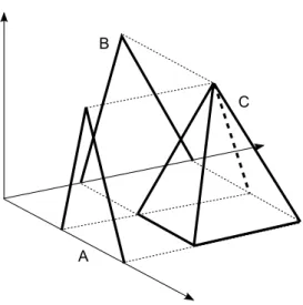
As a special case we define the joint possibility distribution of two fuzzy numbers (see Fig. 1), because we investigate the measures of dependence between pairs of fuzzy numbers.
Definition 2.3. A fuzzy setCinR2is said to be a joint possibility distribution of fuzzy numbersA, B, if it satisfies the relationships
A(x) = max{C(x, y)|y∈R}, and B(y) = max{C(x, y)|x∈R}, (2) for allx, y∈R. Furthermore,AandBare called the marginal possibility distribu- tions ofC.
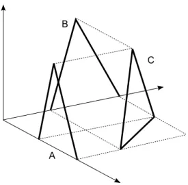
Fuzzy numbersA1, . . . , Anare said to be non-interactive if their joint possibility dis- tributionCsatisfies the relationship
C(x1, . . . , xn) = min{A1(x1), . . . , An(xn)}, for allx= (x1, . . . , xn)∈Rn(see Fig. 2).
Definition 2.4. Aγ-level set (orγ-cut) of a possibility distributionCis a non-fuzzy set denoted by[C]γand defined by
[C]γ =
{(x, y)∈R2|C(x, y)≥γ} ifγ >0
cl(suppC) ifγ= 0 (3)
wherecl(suppC)denotes the closure of the support ofC.
3 Measures of Possibilistic Dependence
3.1 Possibilistic Correlation
Carlsson and Full´er introduced a definition of possibilistic mean and variance [2], and then Full´er and Majlander gave the definition of weighted possibilistic mean and vari- ance [9]. Full´er, Mezei and V´arlaki introduced a new definition of possibilistic correla- tion coefficient [10] between marginal distributions of the joint possibility distribution that improves the earlier definition introduced by Carlsson, Full´er and Majlender [3].
Definition 3.1 (see [10]). Let f: [0,1] → Ra non-negative, monotone increasing function with the normalization property R1
0 f(γ)dγ = 1. The f-weighted possi- bilistic correlation coefficient of fuzzy numbers AandB (with respect to their joint distributionC) is defined by
ρf(A, B) = Z 1
0
ρ(Xγ, Yγ)f(γ)dγ, (4) where
ρ(Xγ, Yγ) = cov(Xγ, Yγ) pvar(Xγ)p
var(Yγ),
and, whereXγ andYγ are random variables whose joint distribution is uniform on [C]γ for allγ∈[0,1], andcov(Xγ, Yγ)denotes their probabilistic covariance.
As we can see, thef-weighted possibilistic correlation coefficient is thef-weighted average of the probabilistic correlation coefficientsρ(Xγ, Yγ)for allγ∈[0,1]. Since f is an increasing function, it gives less importance to the lower levels of the possibil- ity distribution. For detailed and illustrated examples see [8][11] and [12].
The range of thef-weighted possibilistic correlation coefficient when the marginal possibility distribution have the same membership function was discussed in [19] and [17].
Fuzzy numbersA andB are in perfect correlation [3], if their joint distribution is concentrated along a line (see Fig. 3 and Fig. 4), i.e. if there exista, b ∈R,a 6= 0 such that their joint possibility distribution is
C(x1, x2) =
A(x1) ifx2=ax1+b 0 otherwise
B
A
C
Figure 1: Joint possibility distributionCand its marginal possibility distributions (i.e.
projections) fuzzy numbersAandB.
B
A
C
Figure 2: Joint possibility distribution C and its marginal possibility distributions fuzzy numbersAandB when the joint distribution is defined bymin(A, B). In this caseAandBare non-interactive which impliesρf(A, B) = 0.
B
A
C
Figure 3: Joint possibility distributionCand its marginal possibility distributionsA andBwhen the joint possibility distribution is defined along a line with positive steep- ness. This is the case of perfect positive correlation, which impliesρf(A, B) = 1.
B
A
C
Figure 4: Joint possibility distribution C and its marginal possibility distributions A and B when the joint possibility distribution is defined along a line with neg- ative steepness. This is the case of perfect negative correlation, which implies ρf(A, B) =−1.
IfAandB have a perfect positive (negative) correlation then fromρ(Xγ, Yγ) = 1 (ρ(Xγ, Yγ) = −1) (see [3] for details), for allγ ∈ [0,1], we get ρf(A, B) = 1 (ρf(A, B) =−1) for any weighting functionf.
We should note here that while non-interactivity implies zero correlation, the reverse direction is not necesseraly true, if the value of possibilistic correlation coefficient is zero then this not means automatically non-interactivity. For example, if for every γ,[C]γ is symmetrical to an axes which parallel with one the coordinate axis then cov(Xγ, Yγ) = 0andρf(A, B) = 0for any weighting functionf (see [6]).
3.2 Correlation Ratio Between Fuzzy Numbers
The correlation ratioηwas firstly introduced by Karl Pearson [32] as a statistical tool and it was defined to random variables by Kolmogorov [24] as,
η2(X|Y) = D2[E(X|Y)]
D2(X) ,
whereX andY are random variables. It measures not only a linear, but in general a functional dependence between random variablesX andY. IfX andY have a joint probability density function, denoted byf(x, y), then we can computeη2(X|Y)using the following formulas
E(X|Y =y) = Z ∞
−∞
xf(x|y)dx
and
D2[E(X|Y)] =E(E(X|y)−E(X))2, where,
f(x|y) = f(x, y) f(y) .
In 2010 Full´er, Mezei and V´arlaki introduced the definition of possibilistic correlation ratio for marginal possibility distributions (see [7]).
Definition 3.2. Let us denoteAandBthe marginal possibility distributions of a given joint possibility distributionC. Then the f-weighted possibilistic correlation ratio ηf(A|B) of marginal possibility distributionA with respect to marginal possibility distributionBis defined
ηf2(A|B) = Z 1
0
η2(Xγ|Yγ)f(γ)dγ
whereXγ andYγ are random variables whose joint distribution is uniform on[C]γ for allγ∈[0,1], andη(Xγ|Yγ)denotes their probabilistic correlation ratio.
3.3 Informational Coefficient of Correlation
Definition 3.3. For any two continous random variablesX andY (admitting a joint probability density), their mutual information is given by
I(X, Y) = Z ∞
−∞
Z ∞
−∞
f(x, y) ln f(x, y)
f1(x)·f2(y)dxdy
where f(x, y) is the joint probability density function ofX and Y, and f1(x)and f2(y)are the marginal density functions ofXandY, respectively.
Definition 3.4. [27] For two random variables X and Y, let denoteI(X, Y)the mutual information betweenX andY. Their informational coefficient of correlation is given by
L(X, Y) =p
1−e−2I(X,Y).
Based on the definition above, we can define the following [13][14]:
Definition 3.5. Let us denote A and B the marginal possibility distributions of a given joint possibility distributionC. Then the f-weighted possibilistic informational coefficient of correlationof marginal possibility distributionsAandBis defined by
L(A, B) = Z 1
0
L(Xγ, Yγ)f(γ)dγ
whereXγ andYγ are random variables whose joint distribution is uniform on[C]γ for allγ∈[0,1], andL(Xγ, Yγ)denotes informational coefficient of correlation, and f is a weighting function.
There are several other ways to translate the fundamental notions of probability theory to fuzzy numbers (or possibilistic variables), so there are different interpretations for the mean, variance and covariance of fuzzy numbers. Fuzzy random variables are discussed in [26][34] and [33], the variance of fuzzy random variables in [25][31], variance and covariance studied in [5].
Mean value of fuzzy numbers was defined in [4] and [20], the notion of independence is studied in [1], [21] and [35], and with applications in [29], [30].
Liu and Kao [28] used fuzzy measures to define a fuzzy correlation coefficient of fuzzy numbers and they formulated a pair of nonlinear programs to find theα-cut of this fuzzy correlation coefficient, then, in a special case, Hong [22] showed an exact calculation formula for this fuzzy correlation coefficient.
In [15] Full´er et al. introduced a method as a generalization of the concept described in [10]. Here theγ-level sets are equipped with non-uniform probability distribution, whose density function is derived from the joint possibility distribution.
4 Joint Possibility Distribution for Given Correlation
In this section we show a simple way to construct a joint possibility distribution (and in this way marginal possibility distributions) for a given value of the possibilistic correlation coefficient. We recall the fact in probability theory that for any value be- tween−1 and1there exists a 2-dimensional Gaussian distribution whose marginal distributions has this value as correlation coefficient between them (for other types of distributions it is not necesseraly true).
Let the required value of the possibilistic correlation coefficient beρ. Define the joint possibilistic distribution as follows:
C(x, y) = exp
−1
2(1−ρ2)·(x2−2ρxy+y2)
(5) Theγ-level set (remember that0< γ≤1, solnγ≤0):
[C]γ =
(x, y)∈R2|x2−2ρxy+y2≤ −2(1−ρ2)·lnγ (6) Theγ-level set is a (maybe skew) ellipse, whose upper and lower curves are
y1=ρx+p
1−ρ2·p
−2 lnγ−x2 (7) y2=ρx−p
1−ρ2·p
−2 lnγ−x2 (8) The area of theγ-levels set isTγ =−2πp
1−ρ2·lnγ. According to the definition of possibilistic correlation coefficient, we define a two dimensional uniform distribution on theγ-level set, so its density function is
f(x, y) =
1
Tγ if(x, y)∈[C]γ 0 otherwise
(9)
Xγ andYγ are its marginal random variables. The marginal density function ofXγ
(Yγhas the same one):
f1(x) =
−p
−2 lnγ−x2
π·lnγ if−√
−2 lnγ < x <√
−2 lnγ
0 otherwise
(10)
The expected values are
M(Xγ) =M(Yγ) = 0 (11)
M(Xγ2) =M(Yγ2) = −lnγ
2 (12)
M(Xγ·Yγ) = −ρ·lnγ
2 (13)
So the correlation coefficient at levelγ:
ρ(Xγ, Yγ) = cov(Xγ, Yγ) pvar(Xγ)p
var(Yγ) =−ρ·lnγ/2
−lnγ/2 =ρ (14) Since the value ofρnot depends onγ, the value of possibilistic correlation equals this value:
ρf(A, B) = Z 1
0
ρ(Xγ, Yγ)f(γ)dγ=ρ Z 1
0
f(γ)dγ=ρ (15) Note 4.1. In fact the starting point was a two dimensional Gaussian probability den- sity function:
f(x, y) = 1 2πp
1−ρ2·exp
−1
2(1−ρ2)·(x2−2ρxy+y2)
(16)
, whereρis the correlation coefficient between the marginal random variables. So the result we get tells us that the possibilistic and probabilistic correlation coefficient could be the same for certain cases.
5 Correlation Coefficient for t-norm Defined Joint Distributions
An interestinq question is the range or behaviour of the possibilistic correlation coef- ficient when the joint possibility distribution has a special structure, i.e. it is defined by at-norm. According to our best knowledge there are no simple general results to this problem. For the most widely usedt-norm, the minimumt-norm the answer is straightforward, since this is the case when the marginal distributions (fuzzy numbers) are in non-interactive relation and this fact ensures zero correlation coefficient.
The case when the joint possibility distribution is defined by the productt-norm was discussed in [12], where the authors pointed out that the value of the possibilistic correlation falls between−1/2and1/2, including the limits.
Well-known that the following inequality holds for anyt-norm:
Tw(a, b)≤t(a, b)≤min(a, b) (17) whereTwdenotes the weak (or drastic)t-norm:
Tw(a, b) =
min(a, b) ifmax(a, b) = 1,
0 otherwise. (18)
In the following we give strict bounds for the possibilistic correlation coefficients when the joint distribution C(x, y) = Tw(A(x), B(y)), where A and B are the marginal distributions.
a1
b1 b2
(a,b)
d d d a2 d
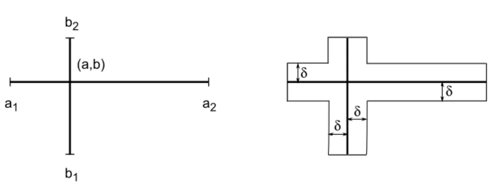
Figure 5: Theγlevel set of the joint distribution, whenC(x, y) = Tw(A(x), B(y)) (left), and itsδneighborhood (right).
Let us denote the core of fuzzy numberAbya, the core ofB byb, theγlevel sets by[a1(γ), a2(γ)]and[b1(γ), b2(γ)], respectively. For simplicity we use the notations:
a1 = a1(γ),a2 = a2(γ), b1 = b1(γ)andb2 = b2(γ). The γ-level sets ([C]γs) of the joint distribution are (not necessarily symmetric) cross-shaped domains (see Fig. 5). The correlation coefficient for this domain is determined as the limit of the correlation coefficient computed for theδneighborhood ([C]γδ) (see Fig. 5). Since the correlation coefficient is invariant under shifting and scaling (multiplying by a positive constant) of the marginal distributions, without loss of generality we can assume that a = b = 0, and−1 ≤ a1, b1 ≤ 0, 0 ≤ a2, b2 ≤ 1, such that at least one of the following conditions hold: a1 = −1, b1 = −1,a1 = −1, b2 = 1,a2 = 1, b2 = 1 ora2 = 1, b1 =−1. These conditions are always feasible: we shift the cores to the origin, then rescaleAbymax{|a1|, a2}andBbymax{|b1|, b2}.
Xγ andYγ are random variables, whose joint distribution is uniform on[C]γδ, the corresponding random variables for[C]γ areXγ0 andYγ0.
The probability density function ofXγ(Yγhas the same with appropriate modification of the parameters):
f1(x) =
1
T·2δ , ifa1< x <−δ;
1
T ·(b2−b1) , if−δ < x < δ;
1
T·2δ , ifδ < x < a2.
whereT = (a2−a1)·2δ+ (b2−b1)·2δ−4δ2denotes the area of[C]γδ.
Computing the expected values and after some simplifications we get:
M(Xγ) = a22−a21
2(a2−a1+b2−b1)−4δ (19) M(Xγ0) = lim
δ→0M(Xγ) = a22−a21
2(a2−a1+b2−b1) (20) M(Xγ2) =2
3·a32−a31+ (b2−b1)δ2−2δ3
2(a2−a1+b2−b1)−4δ (21) M(Xγ02) = lim
δ→0M(Xγ2) =2
3· a32−a31
2(a2−a1+b2−b1) (22)
Similar expressions hold forYγ with appropriate modification of the parameters, of course. The expected value of the product:
M(Xγ·Yγ) = 0 ⇒ M(Xγ0 ·Yγ0) = 0 (23)
The correlation coefficient betweenXγ0 andYγ0:
ρ(Xγ0, Yγ0) = cov(Xγ0, Yγ0) q
var(Xγ0)·q var(Yγ0)
(24)
where
cov(Xγ0, Yγ0) =M(Xγ0 ·Yγ0)−M(Xγ0)·M(Yγ0) = −(a22−a21)(b22−b21) 4(a2−a1+b2−b1)2 (25)
var(Xγ0) = 4
3·(a32−a31)·(a2−a1+b2−b1)−(a22−a21)2
4(a2−a1+b2−b1)2 (26)
var(Yγ0) = 4
3·(b32−b31)·(a2−a1+b2−b1)−(b22−b21)2
4(a2−a1+b2−b1)2 (27)
We prove that the value of the above correlation coefficient always falls between−3/5 and3/5. Let’s consider the case whena2= 1andb2= 1(the estimation works quite similarly for the other three cases). We give a lower estimation for the variances using the fact that−1 ≤a1 ≤0and−1 ≤b1 ≤0, so we get an upper estimation for the
correlation coefficient. The numerator ofvar(Xγ0):
4
3·(1−a31)·(2−a1−b1)−(1−a21)2 (28)
≥ 4
3·(1−a21)2·(2−a1−b1)−(1−a21)2 (29)
= (1−a21)2·
"
4
3·(2−a1−b1)−1
#
(30)
≥(1−a21)2·
"
4 3·2−1
#
= (1−a21)2· 5
3 (31)
Applying this result we get that
var(Xγ0)≥
(1−a21)2·5 3
4(a2−a1+b2−b1)2 (32) So we get the following bounds for the square of the correlation coefficient:
ρ2≤ (1−a21)2(1−b21)2 (1−a21)2·5
3·(1−b21)2·5 3
= 9
25 (33)
which yields:
−3/5≤ρ≤3/5 (34)
These bounds are strict, since
• ifa2=b2= 0anda1=b1=−1, thenρ=−3/5;
• ifa2=b1= 0anda1=−1,b2= 1, thenρ= 3/5.
Remember that the possibilistic correlation coefficient was defined as the weighted average of probabilistic correlation coefficients over the γ levels. We proved that for every γ level set −3/5 ≤ ρ(Xγ, Yγ) ≤ 3/5, so these inequality holds for the possibilistic correlation coefficient for any weighting functionf:
−3/5≤ρf(A, B)≤3/5 (35)
Our numerical and theoretical investigations done so far led us to a conjecture that the weakt-norm has a kind of boundary role here, which is still an open problem:
Question 5.1. Is it true that for any joint possibility distribution defined by at-norm, the possibilistic correlation coefficient falls between−3/5and3/5?
Conclusions
We briefly surveyed the developments of probability relatedγ-level based possibilis- tic measures of dependence. This level-based approach gives a useful tool to directly generalize the notions of probability theory to possibilistic variables and it may make a bridge between possibilistic and probabilistic ways of thinking. Although this con- nection gaves us a chance to adopt the results of probability theory, there are still many open questions.
We gave a short general solution to the inverse problem, namely we showed a family of joint possibility distributions to any given value of correlation. We determined the range of possibilistic correlation coefficient when the joint distribution is defined by the weakt-norm. Finally, we stated an open problem for the family oft-norm defined joint possibility distribution.
Acknowledgement
This work was supported by FIEK program (Center for Cooperation between Higher Education and the Industries at the Sz´echenyi Istv´an University, GINOP-2.3.4-15- 2016-00003).
References
[1] L. M. de Campos, J. F. Huete, Independence concepts in possibility theory: Part I,Fuzzy Sets and Systems103 (1999), pp. 127-152.
Part II.Fuzzy Sets and Systems103 (1999), pp. 487-505.
[2] C. Carlsson, R. Full´er, On possibilistic mean and variance of fuzzy numbers, Fuzzy Sets and Systems122 (2001), pp. 315-326.
[3] C. Carlsson, R. Full´er and P. Majlender, On possibilistic correlation,Fuzzy Sets and Systems, 155(2005) 425-445. doi: 10.1016/j.fss.2005.04.014
[4] D. Dubois and H. Prade, The mean value of a fuzzy number,Fuzzy Sets and Systems, 24(1987), pp. 279-300. doi: 10.1016/0165-0114(87)90028-5
[5] Y. Feng, L. Hu, H. Shu, The variance and covariance of fuzzy random variables and their applications,Fuzzy Sets and Systems120 (2001), pp. 487-497.
[6] R. Full´er and P. Majlender, On interactive possibility distributions, in:
V.A. Niskanen and J. Kortelainen eds., On the Edge of Fuzziness, Studies in Honor of Jorma K. Mattila on His Sixtieth Birthday, Acta universitas Lappeen- rantaensis, No. 179, 2004 61-69.
[7] R. Full´er, J. Mezei and P. V´arlaki, A Correlation Ratio for Possibility Distri- butions, in: E. H¨ullermeier, R. Kruse, and F. Hoffmann (Eds.): Computational
Intelligence for Knowledge-Based Systems Design, Proceedings of the Interna- tional Conference on Information Processing and Management of Uncertainty in Knowledge-Based Systems (IPMU 2010), June 28 - July 2, 2010, Dortmund, Germany, Lecture Notes in Artificial Intelligence, vol. 6178(2010), Springer- Verlag, Berlin Heidelberg, pp. 178-187. doi: 10.1007/978-3-642-14049-5 19 [8] R. Full´er, J. Mezei and P. V´arlaki, Some Examples of Computing the Possibilistic
Correlation Coefficient from Joint Possibility Distributions, in: Imre J. Rudas, J´anos Fodor, Janusz Kacprzyk eds.,Computational Intelligence in Engineering, Studies in Computational Intelligence Series, vol. 313/2010, Springer Verlag, [ISBN 978-3-642-15219-1], pp. 153-169. doi: 10.1007/978-3-642-15220-7 13 [9] R. Full´er, P. Majlender, On weighted possibilistic mean and variance of fuzzy
numbers,Fuzzy Sets and Systems136 (2003), pp. 363-374.
[10] R. Full´er, J. Mezei, P. V´arlaki, An improved index of interactivity for fuzzy numbers,Fuzzy Sets and Systems165 (2011), pp. 50-60.
[11] R. Full´er, I. ´A. Harmati, J.Mezei, P. V´arlaki, On Possibilistic Correlation Co- efficient and Ratio for Fuzzy Numbers, in: Recent Researches in Artificial In- telligence, Knowledge Engineering & Data Bases, 10th WSEAS International Conference on Artificial Intelligence, Knowledge Engineering and Data Bases, February 20-22, 2011, Cambridge, UK, WSEAS Press, [ISBN 978-960-474- 237-8], pp. 263-268.
[12] R. Full´er, I. ´A. Harmati, P. V´arlaki, On Possibilistic Correlation Coeffi- cient and Ratio for Triangular Fuzzy Numbers with Multiplicative Joint Dis- tribution, in: Proceedings of the Eleventh IEEE International Symposium on Computational Intelligence and Informatics (CINTI 2010), November 18- 20, 2010, Budapest, Hungary, [ISBN 978-1-4244-9278-7], pp. 103-108. DOI 10.1109/CINTI.2010.5672266
[13] R. Full´er, I. ´A. Harmati, P. V´arlaki, I. Rudas, On Informational Coefficient of Correlation for Possibility Distributions, Recent Researches in Artificial Intelli- gence and Database Management, Proceedings of the 11th WSEAS International Conference on Artificial Intelligence, Knowledge Engineering and Data Bases (AIKED ’12), February 22-24, 2012, Cambridge, UK, [ISBN 978-1-61804-068- 8], pp. 15-20.
[14] R. Full´er, I. ´A. Harmati, P. V´arlaki, I. Rudas, On Weighted Possibilistic Informa- tional Coefficient of Correlation, International Journal of Mathematical Models and Methods in Applied Sciences, 6(2012), issue 4, pp. 592-599.
[15] R. Full´er, I. ´A. Harmati, P. V´arlaki, Probabilistic Correlation Coefficients for Possibility Distributions, Fifteenth IEEE International Conference on Intelligent Engineering Systems 2011 (INES 2011), June 23-25, 2011, Poprad, Slovakia, [ISBN 978-1-4244-8954-1], pp. 153-158. DOI 10.1109/INES.2011.5954737
[16] R. Full´er, I. ´A. Harmati, P. V´arlaki, On Probabilistic Correlation Coefficients for Fuzzy Numbers, in: Aspects of Computational Intelligence: Theory and Appli- cations: Revised and Selected Papers of the 15th IEEE International Conference on Intelligent Engineering Systems 2011, INES 2011, Topics in Intelligent Engi- neering and Informatics series, vol. 2/2013, Springer Verlag, [ISBN:978-3-642- 30667-9], 2013. pp. 249-263. DOI 10.1007/978-3-642-30668-6 17
[17] R. Full´er, I. ´A. Harmati, On the lower limit of possibilistic correlation coefficient for identical marginal distributions, 8th European Symposium on Computational Intelligence and Mathematics (ESCIM 2016), 2016, C´adiz, pp. 37-42.
[18] H. Gebelein, Das satistische Problem der Korrelation als Variations- und Eigenwertproblem und sein Zusammenhang mit der Ausgleichungsrechnung, Zeitschrift fr angew. Math. und Mech., 21 (1941), pp. 364-379.
[19] I. ´A. Harmati, A note on f-weighted possibilistic correlation for identical marginal possibility distributions,Fuzzy Sets and Systems, 165(2011), pp. 106- 110. doi: 10.1016/j.fss.2010.11.005
[20] S. Heilpern, The expected value of a fuzzy number,Fuzzy Sets and Systems47 (1992), pp. 81-86.
[21] E. Hisdal, Conditional possibilities independence and noninteraction,Fuzzy Sets and Systems1 (1978), pp. 283-297.
[22] D.H. Hong, Fuzzy measures for a correlation coefficient of fuzzy numbers under TW (the weakest t-norm)-based fuzzy arithmetic operations,Information Sci- ences, 176(2006), pp. 150-160.
[23] E.T. Jaynes,Probability Theory : The Logic of Science, Cambridge University Press, 2003.
[24] A.N. Kolmogorov, Grundbegriffe der Wahrscheinlichkeitsrechnung, Julius Springer, Berlin, 1933, 62 pp.
[25] R. K. K¨orner, On the variance of fuzzy random variables,Fuzzy Sets and Systems 92 (1997), pp. 8393.
[26] H. Kwakernaak, Fuzzy random variables–I. Definitions and theorems,Informa- tion Sciences15 (1978), pp. 1-29.
[27] E. H. Linfoot, An informational measure of correlation,Information and Con- trol, Vol.1, No. 1 (1957), pp. 85-89.
[28] S.T. Liu, C. Kao, Fuzzy measures for correlation coefficient of fuzzy numbers, Fuzzy Sets and Systems, 128(2002), pp. 267-275.
[29] X. Li, B. Liu, The independence of fuzzy variables with applications, Interna- tional Journal of Natural Sciences & Technology1 (2006), pp. 95-100.
[30] Y. K. Liu, J. Gao, The independence of fuzzy variables with applications to fuzzy random optimization,International Journal of Uncertainty, Fuzziness &
Knowledge-Based Systems15 (2007), pp. 1-19.
[31] W. N¨ather, A. W¨unsche, On the Conditional Variance of Fuzzy Random Vari- ables,Metrika65 (2007), pp. 109-122.
[32] K. Pearson, On a New Method of Determining Correlation, when One Variable is Given by Alternative and the Other by Multiple Categories, Biometrika, Vol.
7, No. 3 (Apr., 1910), pp. 248-257.
[33] M. L. Puri, D. A. Ralescu, Fuzzy random variables, Journal of Mathematical Analysis and Applications114 (1986), pp. 409-422.
[34] A. F. Shapiro, Fuzzy random variables,Insurance: Mathematics and Economics 44 (2009), pp. 307314.
[35] S. Wang, J. Watada, Some properties ofT-independent fuzzy variables,Mathe- matical and Computer Modelling53 (2011), pp. 970-984.
[36] L. A. Zadeh, Concept of a linguistic variable and its application to approximate reasoning I, II, IIIInformation Sciences8 (1975), pp. 199-249, pp. 301-357;
L. A. Zadeh, Concept of a linguistic variable and its application to approximate reasoning I, II, IIIInformation Sciences9 (1975), pp. 43-80.