Simulation of population distributions of subnational entities (first draft)
P´eter V´ek´as
*April 19, 2020
1 Introduction
Most sovereign countries are divided into administrative divisions. The population distribution of these subdivisions within a country is an important characteristic of national electoral systems.
Supported by theoretical models [Gabaix, 1999], power law distributions were traditionally a frequent choice to describe population sizes of subnational territorial entities. Nevertheless, they have proven to be inadequate in practice on empirical data of cities [Soo, 2004] as well as first-level administrative units [Fontanelli et al., 2017].
Recently, the Discrete Generalized Beta Distribution (DGBD), a broader class of statistical distribu- tions encompassing power laws and several other important special cases, has been used successfully to characterize population sizes of natural cities [Li et al., 2015], countries and their second-level administrative units [Fontanelli et al., 2017], and additionally, the latter paper outlined a model to support its validity.
2 Methods
Instead of the usual cumulative distribution and probability density functions, the Discrete Gener- alized Beta Distribution (DGBD) is customarily defined in terms of its rank-size function, which specifies the relationship between known population sizes x of N entities within a country and the associated population rank numbersrin a descending order [Fontanelli et al., 2017]:1
x(r) =C(N+1−r)b
ra (r=1,2, . . . ,N), (1)
whereaandbare parameters andCis a normalizing constant.
Equation (1) can be fitted to observed population sizes and computed ranks by non-linear regression.
*Corvinus University of Budapest. Address: F˝ov´am t´er 13-15., Room S.201/a, 1093 Budapest, Hungary. Telephone:
+36-1-482-7430. E-mail:peter.vekas@uni-corvinus.hu 1. The special case of power law distributions arises by settingb=0.
1
Fontanelli et al., 2017 describes how to measure the goodness of this fit using a modified version of the Kolmogorov-Smirnov test statistic [Smirnov, 1948] as well as test its statistical significance by bootstrapping [Efron, 1979].
Standard statistical learning techniques such as classification and regression trees [Breiman et al., 1984] and multivariate adaptive regression splines (MARS, Friedman [1991]) may facilitate find- ing groups of countries with a poor fit and predicting the parameters of Equation (1) based on the overall population size and number of subdivisions within a country. In this context, we prefer these two methods to more complex machine learning techniques such as random forests, artificial neural networks or support vector machines due to their superior transparency, interpretability and publisha- bility.
The resulting models may in turn be used to simulate realistic samples of subdivision populations by means of standard random variate generation techniques commonly applied in Monte Carlo simula- tion.
3 Statistical analysis
We used a dataset containing lists of population sizes of all first-level administrative subdivisions of 38 countries for our analysis, which we performed in the R programming language [R Core Team, 2014].
First we applied non-linear regression to estimate the parameters of Equation (1) and thereby fit the DGBD model to each country, and computed theR2values as well as the Kolmogorov-Smirnov test statisticsKSand the associated p-vales of the null hypothesis of a satisfactory fit.
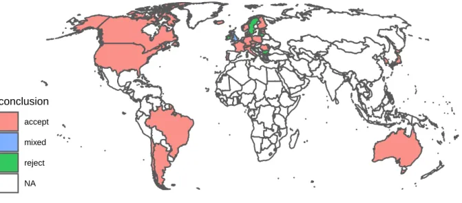
We summarize our results in Figures 1 and 2 as well as Table 1 in the Appendix. The DGBD model fits the data of most countries very well: the meanR2 is 0.94, and the fit may be accepted in 31 out of 38, or equivalently, about 82% of all countries based on the KS test statistics and the associated p-values, assuming the standard significance level ofα =0.05.2 All 7 countries where the fit of the model is not acceptable are located in Europe.
2. Using 1,000 bootstrap samples per country. Increasing the bootstrap sample size did not change the sets of countries where the null hypothesis is accepted or rejected.
Albania
Argentina Australia
Austria Belgium
Brazil
Bulgaria
Canada Chile
Cyprus Croatia
Czechia Denmark
Estonia Finland
France
Germany Iceland
Ireland Italy
Japan Latvia Lithuania
Luxembourg
Malta
Norway Poland
Portugal Romania
Slovenia
South Korea
Sweden Switzerland
England
Wales Northern Ireland Scotland
USA
0.0 0.5 1.0 1.5
−0.5 0.0 0.5 1.0
a
b
conclusion
accept reject
nregions
25 50 75
Figure 1: Estimated DGBD parameters aand b (axes), N (size) and conclusion (color) by country.
The dashed horizontal line atb=0 corresponds to the power law distribution.
conclusion
accept mixed reject NA
Figure 2: Acceptance or rejection of the DGBD model by country
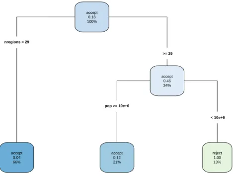
The overall validity of the model can be further enhanced by excluding countries with specific patterns based on their electorate size and number of subdivisions which predispose them to a poor fit. Figure 3 displays a classification tree that identifies a group of this type by predicting the rejection of the null hypothesis of a satisfactory fit.
nregions < 29
pop >= 10e+6
>= 29
< 10e+6 accept
0.18 100%
accept 0.04 66%
accept 0.46 34%
accept 0.12 21%
reject 1.00 13%
Figure 3: Classification tree predicting the rejection of a satisfactory fit
Based on Figure 3, we reject the fit in 100% of the group of countries with at least 29 subdivisions and a total electorate of less than 10 million people, which contains 13% or 5 of all countries ana- lyzed (namely, Bulgaria, Ireland, Lithuania, Scotland and Sweden). These countries can be briefly characterized as having small populations and fragmented systems of subdivisions at the same time.
After excluding these entities from our analysis, as we did, the model became acceptable in 31 out of 33, or equivalently, about 94% of all remaining countries.
As a next step, we used statistical learning techniques to estimate the dependence of the parameters a andb on potentially known predictors: the size of the electorate and the number of subdivisions.
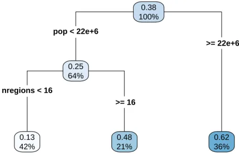
First we fitted a multivariate adaptive regression splines (MARS) model with two independent vari- ables and two predictors, but it returned a non-informative, intercept-only model. Then we built regression trees for the same purpose and optimized them by tuning their complexity using 10-fold cross-validation repeated 10 times. The estimated out-of-sampleR2values of the models are 0.37 for the first tree and 0.53 for the second one: they are far from perfect, but greatly outperform the ’one size fits all’ approach of the intercept-only models. We display the resulting trees in Figures 4 and 5.
pop < 22e+6
nregions < 16
>= 22e+6
>= 16 0.38 100%
0.25 64%
0.13 42%
0.48 21%
0.62 36%
Figure 4: Regression tree predicting the parameteraof the DGBD model
An example of the interpretation of these: if the size of a country’s electorate is less than 22 million people and the number of subdivisions is at least 16 then the estimated value of the parameter a is 0.48 based on the mean value of 21% of all countries used to build the model.
pop < 3.5e+6
nregions >= 14
>= 3.5e+6
< 14 0.52
100%
0.22 27%
0.62 73%
0.41 52%
1.1 21%
Figure 5: Regression tree predicting the parameterbof the DGBD model
To simulate random populations of constituencies, aand bmay be estimated by substituting the size of the electorate and the number of subdivisions into the trees displayed in Figures 4 and 5, and plugging these estimated parameter values and randomly generated ranks into the function defined by Equation (1).
4 Conclusion and limitations
We presented a technique to simulate random subdivision populations based on fitting the DGBD model to data of 38 countries of the world and applying classification and regression trees to predict its potential scope and parameters. The fit of the distribution is excellent, and our method is capable of simulating realistic data, albeit with its own limitations.
The current model only has a high reliability for countries with less than 29 subdivisions or electorates of at least 10 million people, and the trees that predict its parameters assume that the size of the electorate and the number of subdivisions are known.
Our method is confined by the incomplete list of countries it was optimizedon, potential parameter uncertainty, model uncertainty, and the accuracy of the predictions of the regression trees we used to estimate the model parameters.
5 References
Breiman, L., Friedman, J.H., Olshen, R.A., & Stone, C.J. (1984). Classification and regression trees.
Wadsworth & Brooks / Cole Advanced Books & Software, Monterey, CA. ISBN: 978-0-412- 04841-8.
Efron, B. (1979). Bootstrap methods: Another look at the jackknife. The Annals of Statistics, 7(1):1–
26. http://dx.doi.org/10.1214/aos/1176344552.
Fontanelli, O., Miramontes, P., Cocho, G., & Li, W. (2017). Population patterns in World’s ad- ministrative units. Royal Society Open Science, 4(7):170281. https://doi.org/10.1098/
rsos.170281.
Friedman, J. (1991). Multivariate adaptive regression splines. The Annals of Statistics, 19(1):1–67.
http://dx.doi.org/10.1214/aos/1176347963.
Gabaix, X. (1999). Zipf’s law for cities: an explanation. Quarterly Journal of Economics, 114(3):739–767. https://doi.org/doi:10.1162/003355399556133.
Li, X., Wang, X., Zhang, J., & Wu L. (2015). Allometric scaling, size distribution and pattern formation of natural cities. Palgrave Communications, 1:15017. https://doi.org/10.1057/
palcomms.2015.17.
R Core Team (2014). R: A language and environment for statistical computing. R Foundation for Statistical Computing, Vienna, Austria. http://www.R-project.org/.
Smirnov, N. (1948). Table for estimating the goodness of fit of empirical distributions. Annals of Mathematical Statistics, 19(2):279–281. https://doi:10.1214/aoms/1177730256.
Soo, K. (2004). Zipf’s Law for cities: a cross-country investigation. Regional Science and Urban Economics, 35(3):239–263. https://doi.org/10.1016/j.regsciurbeco.2004.04.004.
Appendix
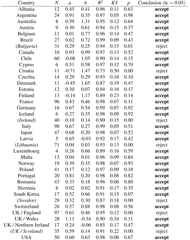
Country N a b R2 KS p Conclusion(α =0.05)
Albania 12 0.45 0.41 0.96 0.11 0.63 accept
Argentina 24 0.91 0.35 0.97 0.05 0.98 accept
Australia 8 0.59 1.31 0.95 0.12 0.64 accept
Austria 9 0.30 0.61 0.94 0.15 0.37 accept
Belgium 11 0.01 0.77 0.96 0.14 0.47 accept
Brazil 27 0.62 0.72 0.99 0.09 0.43 accept
(Bulgaria) 31 0.29 0.25 0.94 0.15 0.01 reject
Canada 10 0.93 0.99 0.97 0.13 0.52 accept
Chile 60 -0.08 1.05 0.90 0.14 0.15 accept
Cyprus 6 0.51 0.58 0.97 0.12 0.70 accept
Croatia 11 -0.71 1.47 0.73 0.50 0.00 reject
Czechia 14 0.29 0.29 0.93 0.16 0.10 accept
Denmark 11 -0.45 1.65 0.87 0.19 0.47 accept
Estonia 12 0.30 0.07 0.94 0.16 0.17 accept
Finland 13 -0.14 1.17 0.89 0.23 0.14 accept
France 96 0.43 0.46 0.98 0.07 0.11 accept
Germany 16 0.67 0.54 0.99 0.07 0.92 accept
Iceland 6 0.27 0.35 0.98 0.09 0.92 accept
(Ireland) 40 0.10 0.14 0.90 0.15 0.00 reject
Italy 98 0.67 0.27 0.99 0.05 0.51 accept
Japan 47 0.68 0.20 0.98 0.07 0.52 accept
Latvia 5 0.65 -0.03 0.92 0.17 0.42 accept
(Lithuania) 71 0.04 0.03 0.93 0.13 0.00 reject
Luxembourg 4 0.26 0.66 0.89 0.16 0.59 accept
Malta 13 0.04 0.01 0.96 0.09 0.84 accept
Norway 19 0.39 0.35 0.98 0.07 0.93 accept
Poland 41 0.17 0.12 0.97 0.09 0.18 accept
Portugal 20 0.81 0.20 0.98 0.08 0.82 accept
Romania 43 0.33 0.18 0.96 0.06 0.80 accept
Slovenia 8 0.02 0.02 0.91 0.17 0.35 accept
South Korea 17 0.52 0.66 0.91 0.15 0.07 accept
(Sweden) 29 0.32 0.30 0.87 0.18 0.00 reject
Switzerland 26 0.57 0.88 0.98 0.08 0.56 accept
UK / England 97 0.61 0.46 0.95 0.12 0.00 reject
UK / Wales 28 1.11 -0.34 0.90 0.34 0.11 accept
UK / Northern Ireland 17 0.24 -0.06 0.85 0.17 0.47 accept (UK / Scotland) 35 0.59 0.14 0.91 0.22 0.00 reject
USA 50 0.60 0.63 0.98 0.06 0.67 accept
Table 1: Fit of the DGBD model by country (names of countries to be excluded from the simulation procedure based on Figure 3 are in parentheses)