THE IMPACT OF EDUCATION EXPENDITURES ON GROWTH IN THE EU28 – A SPATIAL ECONOMETRIC PERSPECTIVE*

(1)

THE IMPACT OF EDUCATION EXPENDITURES ON GROWTH IN THE EU28 –

A SPATIAL ECONOMETRIC PERSPECTIVE*

Lena MALEŠEVIĆ PEROVIĆ

–

Silvia GOLEM

–

Maja MIHALJEVIĆ KOSOR

(Received: 27 September 2016; revision received: 21 February 2017;

accepted: 14 June 2017)

This paper analyses spatial impact of government expenditures on education on economic growth in the EU28 countries during the period 2004–2013. Employing a novel econometric technique that allows for the estimation of spatial spillovers, our results indicate that government expenditures on education signifi cantly and positively infl uence GDP growth. Moreover, the indirect i.e. the spillover effects are quite large suggesting that the growth models should account for spatial interdependencies. Precisely, we fi nd that education expenditures in one country affect GDP growth in the neighbouring countries, meaning that these spillovers are geographical in nature. Moreover, we fi nd that the degree of interdependence among countries varies according to the average GDP per capita even if their geographical distances are identical. Additionally, immigration is found to be an important channel of spatial transmission.

Keywords: government spending on education, GDP growth, spatial panel analysis, spillover ef- fects

JEL classifi cation indices: C33, H1, H5, I2, O4

* The authors thank Giovanni Millo for helpful advices, technical help and support in writing of this paper. This work has been fully supported by Croatian Science Foundation under the project No. UIP-2013-11-9558.

Lena Malešević Perović, corresponding author. Associate Professor at University of Split, Faculty of Economics, Business and Tourism, Croatia. E-mail: lena@efst.hr

Silvia Golem, Assistant Professor at University of Split, Faculty of Economics, Business and Tourism , Croatia. E-mail: sgolem@efst.hr

Maja Mihaljević Kosor, Assistant Professor at University of Split, Faculty of Economics, Business and Tourism, Croatia. E-mail: majam@efst.hr

(2)

1. INTRODUCTION AND MOTIVATION

The Maastricht Treaty and the Stability and Growth Pact (SGP) require national fiscal policies in the euro zone and in the candidate countries to keep their fiscal deficits below 3% of GDP and their public debts below 60% of GDP. In spite of that, the recent global financial and economic crisis has led to fiscal expansions though various fiscal stimulus packages resulting in mounting government deficits and debts worldwide. In order to ensure the long-term sustainability of public finances, policy makers are now forced to curb the size of the government sector.

In such a situation the structure of government spending becomes increasingly important. Namely, provided that different types of government expenditures have different growth effects, the analysis of the composition of government expenditures in relation to the long-run economic growth offers an important basis for relevant policy proposals. Although the governments make spending cuts in order to improve public finances, an attempt to cut down all types of expenditures linearly (i.e. proportionately) might lead into a public-savings paradox whereby non growth-enhancing, that is, unproductive expenditures, crowd out the potential growth-enhancing expenditures (Colombier 2011). In order to avoid this ‘budget crowding out’ effect, policy makers should have a clear guidance on the growth effects of different expenditure types. In that light, this paper adds to the literature by investigating the growth impact of one particular type of productive government expenditures – i.e., the education expenditures.

Governments all around the world have become aware of the importance of their role in the formation of human capital which is recognised as a key driver of productivity, growth and prosperity. The necessity of investing in human capital has been recognised explicitly by the European Commission, whose 2020 strategy has put forward EU targets in the following five areas: employment, research and innovation, climate change and energy, education and poverty reduction (European Commission 2010). Therefore, an investigation of the impact of education expenditures on growth seems particularly appropriate and an up- to-date topic.

Government expenditures on education influence growth through facilitating human capital accumulation. However, it should be noted that in economically integrated economies most economic policies are spatially dependent. The policy choice of one country, region, state or municipality depends partly on policy choices of other countries, regions, states or municipalities. Similarly, as Elhorst (2014) highlights, the economic growth variable is expected to depend not only on the initial income level, the rates of saving, population growth, technological change and depreciation in their own economy, but also on those variables in the neighbouring economies. Even though the recent years have seen a growing

(3)

interest of mainstream econometrics on spatial statistical methods, most empirical studies that investigate government expenditures (at its aggregate and disag- gregate level) and growth nexus ignore spatial aspect of the growth process and the possibility of spatial autocorrelation is rarely acknowledged (Nijkamp – Poot 2004).

Given the above arguments, the main goal of this paper is to analyse the impact of government’s education expenditures on growth in the EU28 countries during 2004-2013 using the spatial econometrics approach. We hypothesise that GDP growth in one country depends not only on population, physical and human capital (approximated by education expenditures) in that country, but also on population, physical and human capital in other countries which can be considered as

“close” in either geographical or economic terms.

This paper, thus, complements and extends the literature in several ways. First- ly, unlike the majority of the papers on this topic we take into account possible spatial dependencies among countries in the sample. As noted by Abreu et al.

(2004), the possibility that space is a determinant of growth has been considered in several papers, which mostly use geographical variables, while spatial econometrics literature has concentrated primarily on regional data instead of country data. Ignoring the spatial issues can lead to misestimated standard errors (Anselin – Griffith 1988); hence, in the presence of spatial dependence, traditional (a-spatial) econometric techniques are no longer appropriate. Thus, by using a more appropriate estimation technique we are able to address some important methodological issues (cross sectional dependence in general and spatial dependence in particular) which impair the findings of the previous empirical studies.

Furthermore, we test the channels of spatial transmission – this issue has not been investigated in the education expenditure-growth relationship before. Precisely, we investigate whether education spillovers exist, and if so whether they are only geographical in nature, i.e. mostly felt by nearest neighbours, or economic relationships play a role. In doing this we test various spatial weights matrices and different spatial econometrics models. We find that GDP growth in one country depends on, among other things, education expenditures in neighbouring countries, with a distance-decay effect. Moreover, the degree of inter-country dependence varies according to the economic relationships between the countries even if geographical distances are identical. Immigration in particular is found to be an important channel of spatial transmission.

The paper is organised as follows: Section 2 gives theoretical background for the empirical model that will be used for the analysis; Section 3 reviews empirical literature on the topic; Section 4 presents methodological approach undertaken in this paper; Section 5 gives the results as well as robustness tests, while Section 6 concludes.

(4)

2. THEORETICAL BACKGROUND

The theoretical growth model that our empirical estimation will be based upon is spatially augmented Mankiw et al.’s (1992) model. Fisher (2011) extends this model by accounting for spatial externalities caused by the disembodied knowledge diffusion and links theory and empirical testing through the Spatial Durbin model (SDM) to test interregional differences in output per worker.

Mankiw et al.’s (1992) model, which is in effect, Solow’s (1956) model augmented with human capital as a separate input in the production function, provides an excellent description of the cross-country data and is consistent with the international evidence. The three key variables (human and physical capital and population growth) account for approximately 80 per cent of the cross-country variation in income. In this model human capital is assumed to be accumulated in the same way as physical capital: by investing a fraction of income in its production. To the extent that government expenditures on education facilitate human capital accumulation (since most governments are involved in the formation of human capital by providing funds for education) there is a scope for governments to influence long-run growth. Therefore, we assume that government expenditures on education are represented through the human capital variable.

In Fisher’s (2011) model, a starting point is the Cobb-Douglas production function of the following form:

K H 1 K H

it it it it it

Y A K H L^α ^α ^^α ^^α (1) with standard notations: for country i at time t, Y is the output, K is the level of physical capital, H is the level of human capital, L is the level of labour and A is the level of technological knowledge. α_K and α_H are output elasticities with respect to K and H, respectively. They are assumed to be positive, with decreasing returns to both types of capital.

The key addition to Mankiw et al.’s (1992) model is that Fisher (2011) assumes that each unit of capital investment increases not only the stock of physical capital but also the level of technology of all firms in the economy through knowledge spillover. Moreover, it is assumed that these externalities are not constrained by region borders and that the technological progress of one region positively depends on technological progress of other regions, but with diminished intensity.

Fisher (2011) follows Ertur – Koch (2007) in this, but broadens their model with human capital. This results in the following function that describes the aggregate level of technology:

Ù ^N ^W^ij.

it t it it jt

j i

A k h^θ ^ A^γ







(2)

(5)

The function given in (2) depends on four terms. Ω_t is the common stock of knowledge i.e. a proportion of technological progress which is exogenous and identical in all countries. Furthermore, each country’s level of technology increases with the aggregate level of physical capital per worker, k^θ_it, as well as with the aggregate level of human capital per worker, h^ϕ_it. Technical parameters θ and ϕ reflect spatial connectivity of k_itand h_it within region i, respectively. Finally, the term



^N_{j i}_A^γ_jt^W^ij is a geometrically weighted average of stock of knowledge of a country’s neighbours (denoted by j). Within this term, W_ijis the spatial weights matrix which captures spatial connectivity between the regions and γ reflects the degree of regional interdependence.

For the space-preservation reasons we do not develop the whole model here;

rather we present only the reduced form theoretical model ¹:

 

*

1 Ù

1 1 1 1 1

1

1 1 1

K H N K

K H K

it t i i i ij j

j i

N N N

H H K H K H

ij j ij i ij jt

j i j i j i

lny ln lns lns ln n g W lns

W lns W ln n g W lny

α θ α η δ α γ

η η η η η

α α α α α

γ γ δ γ

η η η



  

  

       

    

  

   

  



  

⁽³⁾

where s^K_i and s^H_iare investment rates of physical and human capital, respectively;

δ is the rate of depreciation of both stock of capital; n is the rate of population growth; g is the growth rate of technology and η α _K α_H   θ .

According to equation (3), the regions with higher output per worker will be those that have higher investment rates in physical and human capital, and lower rates of population growth and depreciation. This is in line with the implications of the Mankiw et al. (1992) model. A novel conclusion that can be derived from this model, however, is that output per worker in region i also depends on growth determinants from other regions. Equation (3) implies that this output will be negatively affected by investment rates in physical and human capital in neighbouring regions j, and positively by their rates of population growth. Empirical counterpart of Fisher’s (2011) theoretical model as given in equation (3) will be presented and used in our empirical analysis in Section 4.

Although Fisher’s (2011) model is developed to assess the role played by regional technological interdependence in the growth process, we use this model at the country level. This is in line with Ertur – Koch (2007), who developed a theoretical growth model which accounts for technological interdependence between countries and estimates the spillover effects; whereby technological interdependence is assumed to work via spatial externalities. They argue that a

1 Equation (3) is derived from equations (1) and (2) according to Fisher (2011: 423–425).

(6)

model needs to include these interdependencies in order to explain growth, as the knowledge accumulated in one country depends on the knowledge accumulated in other countries. In their analysis the intensity of spillover effects is captured by geographical proximity and found to be decreasing with distance. Overall, they conclude that countries cannot be treated as spatially independent observations, and that growth models should account for these spatial interactions explicitly.

3. LITERATURE REVIEW

As for the empirical counterpart of the growth models that take into account technological interdependencies among economies in the form of spatial externalities due to knowledge diffusion, not many studies have been undertaken. Pede et al.

(2008) first estimate the simple Solow growth model, then the augmented Solow model with human capital, and given that there was an overwhelming evidence of spatial autoregressive process, finally the Mankiw et al. (1992) model with spatial regimes. The data used to operationalise and estimate the Mankiw et al.

(1992) model are for 3074 counties of the contiguous 48 states of the U.S., di- vided in the high- and the low-income groups, and the time period covered is 1969-2003. All data series are averaged over the entire time period. The results for the two groups are fairly similar with the exception of the population growth variable, which is positive but insignificant for the high-income group. Also, the Chow test suggested that the high and the low initial income regions exhibit different speeds of convergence as well as different steady states, which is in line with Mankiw et al. (1992) suggesting that human capital strongly contributes to economic growth. The rate of human capital accumulation was defined as the proportion of the population aged 25 years and older with at least a 4-year col- lege degree. For both the groups, the human capital variable is positive and highly significant. Their empirical analysis also includes examination of a growth model which is not directly comparable to Mankiw et al. (1992) model; rather it is an endogenous growth model that represents an extension of Nelson – Phelps (1966) and Benhabib – Spiegl (1994) models. The authors extend the original Benhabib – Spiegl (1994) model by incorporating a spatial spillover effect for the human capital stock and a distance decay effect in the catch-up process. The results show that human capital contributes to growth, but the effect is weaker compared to the Mankiw et al. (1992) growth setting. For the high-income regions, the results suggest that the effect of human capital is positive and significant, and that the spatial spillover effect of human capital of the neighbouring regions is positive, but not significant. For the low-income group, the letter effect is negative and barely significant. Similarly, Máté (2015) measures the impact of human capital

(7)

in an extended Mankiw et al. (1992) model, and finds that it is negatively correlated with the productivity growth in the low-skilled sectors.

In the empirical part of his study, Fischer (2011) assesses the importance of cross-region technological interdependence and measures both direct and indirect (spillover) effects of the three Mankiw et al. (1992) determinants – physical capital, human capital and labour – on regional output using a reduced-form SDM specification. They employ a system of 198 regions across 22 (Western and Eastern) European countries, averaged over the period 1995–2004. The finding of positive and significant spatial autocorrelation indicates that the regions cannot be treated as independent observations and suggests that the growth models should explicitly account for the technological interdependence. In this study human capital is measured in terms of educational attainment based on data for the active population aged 15 years and older that attained the level of tertiary education. The estimated SDM model indicates that the direct estimated impact of the human capital variable is positive and statistically significant. The indirect impact of spatial spillovers of human capital is negative, but statistically insignificant. Hence, the results suggest the absence of cross-region human capital spillovers. However, the results further indicate the existence of cross-region physical capital spillovers, suggesting that interdependence among regions works through the physical capital externalities. The authors point out that this finding does not imply that the role of human capital is unimportant. Even using an im- precise proxy for human capital, the study finds that human capital investment is important – a 10% increase in human capital investment leads to a 1.5% increase in regional output, and this increase is statistically significant.

Lima – Neto (2015) also use a spatial extension of the Mankiw et al. (1992) model to identify the determinants of economic growth for a panel of 522 Brazil- ian micro-regions over the period 1970–2010. They employ a SDM with fixed-effects, an empirical strategy that simultaneously considers the spatial dependence and specific heterogeneity of each economy. The results indicate a strong spatial dependence among Brazilian micro-regions and that investments in both physical and human capital are important for the growth of the Brazilian regional economies. Namely, the results suggest that human capital - measured as the average years of schooling of the population over 25 years of age – and physical capital generate positive and statistically significant spillover effects. With respect to the obtained magnitudes of the direct and the indirect impacts, one standard devia- tion increase in human and physical capital investment in an economy generate similar variations in growth, while the latter exhibits a slightly larger impact.

Cravo et al. (2015) also examine the main determinants of economic growth for a panel of 508 Brazilian micro-regions for the period 1980–2004, using spatial econometrics, but focusing more on a role played by small and medium-size en-

(8)

terprises (SMEs). Their results indicate that human capital level of the whole population is an important growth determinant; however, there are no significant positive spillovers. Furthermore, human capital embodied in SMEs is more important than the size of this sector for regional growth but does not generate positive spatial spillovers.

Paas – Schlitte (2009) investigate income convergence in the EU countries and their NUTS3 level regions, taking into account spatial interactions and control- ling for spatial autocorrelation. Building upon the work of Barro – Sala-i-Martin (1992), to estimate regional income convergence they specify and estimate two types of spatial models – Spatial Lag Model and Spatial Error Model. The results suggest that the spatial growth spillovers play an insignificant role and imply that the national macroeconomic factors exert a greater influence on regional growth than the spatial interactions. The spatial growth spillovers seem to stop at national borders, which indicate that border impediments still matter for the intensity of economic cross-border integration in the EU.

There are some papers that investigate the relationship between government’s educational expenditures and growth in an a-spatial manner. Baldacci et al. (2004) use a system of equations and investigate the direct and the indirect channels between social spending, human capital and economic growth. They find that education and health expenditures have a significant and positive direct impact on economic growth. Bose et al. (2007) explore the impact of disaggre- gated government expenditures on growth. They find that education is the key sector for growth. Afonso – Gonzalez Alegre (2008) test whether the reallocation of government budget items influences long-term economic growth, total factor productivity and labour productivity, in turn. Using a dynamic panel data model with lags of explanatory variables they find that government consumption and social security contributions influence long-term growth negatively while the impact of government investment is positive. Government expenditures on education are found to be growth-enhancing. Acosta-Ormaechea – Morozumi (2013) investigate how changes in the composition of government expenditures affect long-run growth. Their analysis reveals that only educational expenditures have statistically significant growth-enhancing effects. Gemmell et al. (2014) investigate the influence of total government expenditures as well as of composition of government expenditures on the long-run GDP levels. Using a pooled mean group (PMG) approach, they find that keeping total expenditures unchanged, the increases in the share of transport and communication and education in GDP (off- set by pro-rata reduction in other types of spending) lead to increases in GDP per capita in the long-run. All of the above mentioned studies point to a positive relationship; however, neither one of them has accounted for spatial effects; hence, the results should be interpreted cautiously.

(9)

4. METHODOLOGICAL APPROACH AND DATA

Given the theoretical discussion in Section 2, the empirical model used for our analysis stems from theoretical model as given by equation (3). The empirical counterpart of this model (for details how to derive equation (4) from equation (3) please see Fisher 2011) is the SDM given as:

it it it it i it

y ρWy βx θWx  a u (4) where y_it is the dependent variable for country i at time t, ρ is the spatial autocorrelation coefficient, W is the spatial matrix for the autoregressive component, x_it is a set of independent variables, θ is a vector of the regression parameters associ- ated with spatially-lagged exogenous variables, a_i is the individual random effect and u_it is a normally distributed error term. The three independent variables included in our initial model comprise of Mankiw et al.’s (1992) growth regression variables: population growth (Population), physical capital (Investment) and human capital, whereby we approximate human capital with education expenditures (Education), as our main variable of interest. As noted by Nonneman – Vanhoudt (1996), this variable is a closer proxy for direct investment in education, especially for countries such as OECD², where education is systematically subsidised.

In equation (4), Wx represents growth determinants not suggested by the original Mankiw et al. (1992) theory, and so does Wy, which represents the technological interdependence between countries. The estimation method used is maximum likelihood.

The presence of spatial dependence renders the traditional econometric techniques no longer appropriate for spatial data analysis, given that the assumption of independent and identically distributed observations is no longer valid. It is therefore crucial to use the appropriate econometric techniques that deal with spatial interactions among the geographical units. In estimating the relationship between government expenditures on education and growth we, therefore, apply the (static) spatial panel model given that our sample consists of 28 (EU) countries and 10 years (2004–2013) observations. The number of years is dictated by the fact that the spatial empirical approach requires panels to be balanced, and the data for years prior to 2004 proved to be unobtainable in some cases. Table 1 gives an overview of the variables used in terms of definition and data sources, while Table 2 presents their descriptive statistics.

One of the key issues in the spatial econometrics literature is the shape, i.e.

definition of the spatial weights matrix. In general, it is a N by N non-negative matrix which expresses for each observation (row) those locations (columns) that

2 The same can be concluded for the EU countries.

(10)

belong to its neighbourhood, set as the nonzero elements (Anselin – Bera 1998).

There are various options regarding the shape of this matrix, some of which take into account only geographical proximity of the units under investigation, while some other account also for social, economic and similar linkages. Since the majority of the literature assumes that geographic measures are decisive in determin- ing the degree of interaction across countries, in our baseline specification we use a row-standardized 1-nearest neighbour spatial weights matrix (wknn1). Later on we test the robustness of our results by changing the definition of this matrix.

5. RESULTS

Before embarking upon estimation of equation (4), we check if spatial correlation exists by testing for cross-sectional dependence. It is to be expected that countries are cross-correlated due to the economic and financial integration among them and/or common macroeconomic shocks. Ignoring these cross-correlation results in inefficient parameter estimates is likely to lead to size distortions of conven- tional tests of significance. Therefore, first we apply the Pesaran (2004) cross- sectional dependence (CD) test (global CD test) for each variable. The results in Table 3 suggest that in all the cases except for the population variable, the null of cross-sectional independence is rejected.

Table 1. Definitions and sources of the variables

Variable Indicator(s) Source GDPpc_growth Difference in log of real GDP at constant 2011

national prices (in mil. 2011US$) Feenstra et al. (2015) Investment Share of gross capital formation at current PPPs in

GDP Feenstra et al. (2015)

Population Difference in log of population (in millions) Feenstra et al. (2015) Education • Government expenditure on education (% of total

government expenditure) Eurostat (2016)

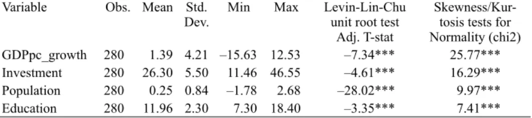
Table 2. Descriptive statistics Variable Obs. Mean Std.

Dev. Min Max Levin-Lin-Chu unit root test

Adj. T-stat

Skewness/Kur- tosis tests for Normality (chi2) GDPpc_growth 280 1.39 4.21 –15.63 12.53 –7.34*** 25.77***

Investment 280 26.30 5.50 11.46 46.55 –4.61*** 16.29***

Population 280 0.25 0.84 –1.78 2.68 –28.02*** 9.97***

Education 280 11.96 2.30 7.30 18.40 –3.35*** 7.41***

Note: ^* p < 0.10, ^** p < 0.05, ^*** p < 0.¹01.

(11)

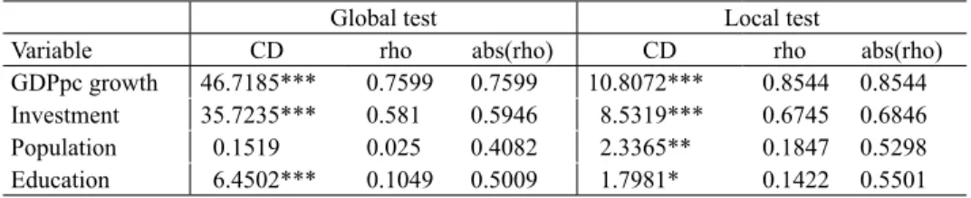
Next we test whether this cross-sectional dependence is characterised by spatial patterns. The spatial dependence is a special case of cross-sectional dependence in the sense that it occurs when cross-sectional correlations follow a certain type of spatial ordering which characterises the neighbour relation. For this we use the local variant of the CD test called the CD(p) test (Pesaran –Tosetti 2011) (local CD test) that takes into account the spatial weights matrix to test the null of no cross-sectional dependence against the alternative of local cross-sectional dependence. As can be seen from Table 3 the null of cross-sectional independence is again rejected, suggesting local dependence, i.e. dependence between the neighbours only. This means that the cross-sectional correlation can be treated as spatial correlation. The rho (ρ) and abs(rho) in Table 3 are descriptive statistics. The first is the simple average of pairwise correlation coefficients between the cross-sectional units, while the second is the average of the absolute values thereof. All of the undertaken tests suggest the presence of spatial dependencies.

Moreover, the tests of the whole model for cross-sectional correlation of either global or local nature (not reported but available upon request) indicate that we can reject the null of cross-sectional independence. The application of spatial econometric techniques is, therefore, justifiable.

Table 4 (column 1) provides an estimation of the SDM model, as given by equation (4) with W created as row-standardised 1-nearest neighbour spatial weights matrix (wknn1) of the size (28×28). The SDM is our initial empirical specification since it is derived from a theoretical model given in Section 2. How- ever, in order to determine whether the SDM presents the best fit for the data, we also test another two spatial models. The first one is the Spatial Autoregressive (SAR) model (Table 4, column 2), which is given as:

it it it i it.

y ρWy βx  a u (5) The SAR (equation 5) is nested within the SDM (equation 4), since in the SDM both the dependent and the independent variables are spatially lagged, where- as in the SAR model the interaction effects among the exogenous independent variables are not significant. In order to determine the ‘true’ spatial process we

Table 3. Test for global and local cross-sectional dependence in variables

Global test Local test

Variable CD rho abs(rho) CD rho abs(rho)

GDPpc growth 46.7185*** 0.7599 0.7599 10.8072*** 0.8544 0.8544 Investment 35.7235*** 0.581 0.5946 8.5319*** 0.6745 0.6846

Population 0.1519 0.025 0.4082 2.3365** 0.1847 0.5298

Education 6.4502*** 0.1049 0.5009 1.7981* 0.1422 0.5501

Note: ^* p < 0.10, ^** p < 0.05, ^*** p < 0.01.

(12)

undertake the log likelihood test by testing the hypothesis that θ = 0. The results (p-value=0.41) suggest non-rejection of the null, thus favouring the SAR model.

We also test the Spatial Error Model (SEM) (Table 4, column 3), given as:

it it i it

it it it

y x a v

v Wv u

β λ

  

  (6) where λ is the coefficient on the spatially correlated errors. This model assumes that the spatial correlation comes only through the error term, i.e. the units of observation are cross-correlated only through shocks in neighbouring units. In order to determine whether the SEM is preferable to the SDM, we test the hypothesis that θ = –ρβ. The rejection of the null (p-value=0.000) provides statistical evidence in favour of the SDM. Finally, we choose between the fixed and the random effects model using the Hausman test. The Hausman test suggests that the fixed effects are preferred to the random effects. Additionally, since we do not want to draw conclusions outside our sample, i.e. population can be considered to be sampled exhaustively as all the EU28 countries are included, the fixed effects model makes more sense. Therefore, for both economic and econometric reasons, we opt for the fixed effects model.

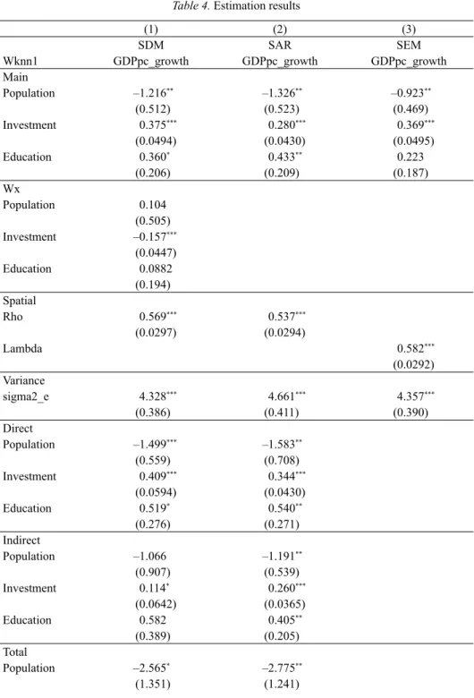
The results in Table 4 suggest the following. Firstly, all of the estimated coefficients have the expected signs and are statistically significant (except for Educa- tion in the SEM). More precisely, Investment and Education are found to exert a positive impact on GDP per capita growth and a negative impact on Population.

In the SDM (column 1) the direct effects of Investment, Population and Educa- tion are statistically significant and of expected signs, while the indirect effects are significant for Investment only. The spatial lag coefficients, Wx are also found to be statistically non-significant, except for Investment. This is in line with our previous finding that the SDM can be reduced to the SAR model.

As for the SAR model (column 2), the signs on all of the variables are in line with expectations, i.e. positive on Investment and Education and negative on Population. As noted by LeSage – Pace (2009), interpretation of the obtained coefficients is not as straightforward as in the linear regressions, since the spatial regression models additionally include information from neighbouring regions/

observations. In these models one can differentiate between the “direct” and the

“indirect” effects, while the “total“ average effect of a change in an independent variable on the dependent variable is the combination of the two. In our case, the direct effect measures the influence of changes in fundamentals within one country on its own GDP growth, once the spatial multiplier is accounted for. The indirect effect measures the influence of changes in other countries’ explanatory variables (fundamentals) on GDP growth of a certain country. The main estima-

(13)

Table 4. Estimation results

(1) (2) (3)

SDM SAR SEM

Wknn1 GDPpc_growth GDPpc_growth GDPpc_growth

Main

Population –1.216^** –1.326^** –0.923^**

(0.512) (0.523) (0.469)

Investment 0.375^*** 0.280^*** 0.369^***

(0.0494) (0.0430) (0.0495)

Education 0.360^* 0.433^** 0.223

(0.206) (0.209) (0.187)

Wx

Population 0.104

(0.505)

Investment –0.157^***

(0.0447)

Education 0.0882

(0.194) Spatial

Rho 0.569^*** 0.537^***

(0.0297) (0.0294)

Lambda 0.582^***

(0.0292) Variance

sigma2_e 4.328^*** 4.661^*** 4.357^***

(0.386) (0.411) (0.390)

Direct

Population –1.499^*** –1.583^**

(0.559) (0.708)

Investment 0.409^*** 0.344^***

(0.0594) (0.0430)

Education 0.519^* 0.540^**

(0.276) (0.271)

Indirect

Population –1.066 –1.191^**

(0.907) (0.539)

Investment 0.114^* 0.260^***

(0.0642) (0.0365)

Education 0.582 0.405^**

(0.389) (0.205)

Total

Population –2.565^* –2.775^**

(1.351) (1.241)

(14)

tion results are given in the first part of Table 4, while the direct and the indirect spillover effects are given in the lower part of the table. Both these effects in the SAR model are found to be statistically significant. More precisely, Investment is found to have a direct impact of 34.4 basis points for 1 percentage point increase.

Once the indirect effects are taken into account, this impact increases to 60.4 basis points. A 1 percentage point increase in Population growth is found to decrease GDP growth by 158.3 basis points directly, or, overall, by 277.5 basis points.

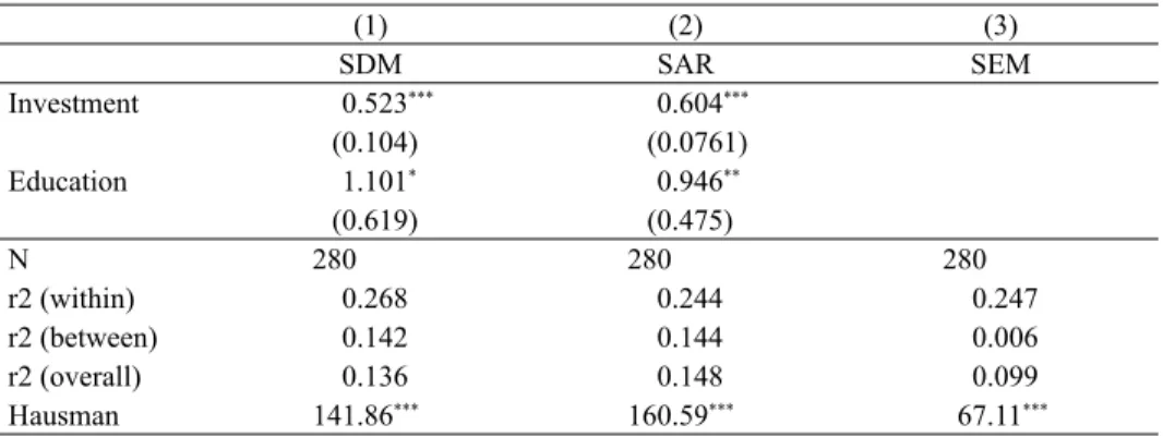
Finally, for Education, our main variable of interest, we find that a 1 percentage point increase in education expenditures in overall government expenditures leads to an increase in GDP growth of 94.6 basis points; 54 of which can be attributed to the direct effects and 40.6 to the indirect ones. Overall, the indirect effects have a large impact accounting for, on average, 43 per cent of the total effect. This finding indicates that the fundamentals in other (neighbouring) countries have significant spatial spillover effects, i.e. a change of education expenditures in one country leads to a change in GDP growth in another (neighbouring) country. In addition, it should be stressed that spatial Rho (ρ), which captures the feedback effects that arise from GDP per capita growth in the neighbouring countries, is statistically highly significant confirming the importance of the spatial effects and suggesting that countries cannot be treated as independent observations.

Furthermore, the differences between the direct effects and the coefficient estimates (given under the title Main in Table 4) are relatively small. These differences are due to the endogenous interaction effects, Wy, which cause the feedback effects. For example, the impacts that are affecting GDP per capita growth in certain countries pass on to the surrounding countries and back to the country where the change first has happened. The direct effect on Education is 0.540, while the coefficient estimate on this variable is 0.433, which implies that the feedback ef-

(1) (2) (3)

SDM SAR SEM

Investment 0.523^*** 0.604^***

(0.104) (0.0761)

Education 1.101^* 0.946^**

(0.619) (0.475)

N 280 280 280

r2 (within) 0.268 0.244 0.247

r2 (between) 0.142 0.144 0.006

r2 (overall) 0.136 0.148 0.099

Hausman 141.86^*** 160.59^*** 67.11^***

Note: Standard errors are in parentheses; ^* p < 0.10, ^** p < 0.05, ^*** p < 0.01; Stata command xsmle is used for all computations.

Table 4. cont.

(15)

Table 5. Robustness check with different spatial weights matrices

(1) (2) (3)

W = winvsq W = wimg W = wecon

SAR GDPpc_growth GDPpc_growth GDPpc_growth

Main

Population –1.228^** –1.388^** –1.353^**

(0.483) (0.577) (0.552)

Investment 0.286^*** 0.419^*** 0.256^***

(0.0390) (0.0454) (0.0439)

Education 0.188 0.443^* 0.373^*

(0.194) (0.231) (0.211)

Spatial

rho 0.826^*** 0.738^*** 0.574^***

(0.0333) (0.0421) (0.0296)

Variance

sigma2_e 3.996^*** 5.699^*** 4.381^***

(0.341) (0.494) (0.408)

Direct

Population –1.431^*** –1.642^*** –1.773^***

(0.470) (0.572) (0.606)

Investment 0.334^*** 0.497^*** 0.338^***

(0.0479) (0.0592) (0.0603)

Education 0.226 0.530^* 0.495^*

(0.236) (0.283) (0.285)

Indirect

Population –5.801^*** –3.770^*** –1.420^***

(2.194) (1.461) (0.497)

Investment 1.358^*** 1.148^*** 0.270^***

(0.323) (0.259) (0.0490)

Education 0.876 1.204^* 0.394^*

(1.003) (0.686) (0.230)

Total

Population –7.232^*** –5.411^*** –3.193^***

(2.610) (1.992) (1.097)

Investment 1.692^*** 1.646^*** 0.608^***

(0.352) (0.301) (0.107)

Education 1.102 1.734^* 0.889^*

(1.234) (0.958) (0.514)

N 280 280 260

r2 (within) 0.252 0.231 0.230

r2 (between) 0.129 0.029 0.166

r2 (overall) 0.231 0.146 0.143

Note: Standard errors are in parentheses; ^* p < 0.10, ^** p < 0.05, ^*** p < 0.01; Stata command xsmle is used for all computations.

(16)

fect is (0.540–0.433=) 0.107. This feedback effect corresponds to approximately 25% of the coefficient estimate.

In the SEM model (column 3) all the variables have the expected signs; however, Education is statistically insignificant. Since this approach corrects only for the efficiency of the estimated coefficients, the indirect and the direct effects are neither calculated nor reported. Spatial Lambda (λ) is statistically highly significant and positive thus confirming the presence of spatial dependence in our data.

Overall, our results so far have shown that the spatial panel model is a better alternative to the a-spatial version of the panel model, and within a set of spatial models the SAR is our preferred specification. Since the SAR is nested within the SDM, this is in line with theoretical background presented in Section 2.

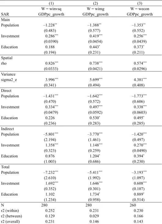
Next, we use different weights matrices to evaluate whether and to what extent our results are sensitive to the structure of these matrices. Moreover, different matrices will allow us to test the channels of spatial transmission.

In column 1 of Table 5 we provide the results of using an inverse distance squared spatial weights matrix (winvsq) which reduces the weight of more distant countries. The results remain largely the same in terms of signs and significances of the tested variables, except for Education, which turns insignificant. In our original specification, when one nearest neighbour spatial weights matrix was used, Education became significant. When two and three nearest neighbour spatial weights matrix is used (unreported but available upon request), Education is also found to be significant. Taken together, our results suggest that the spillovers are felt by the nearest neighbours, but this effect fades away with distance.

So far we have estimated our model by assuming that geographical proximity reflects cross-country linkages and plays a key role in the effect of education (and other fundamentals) on growth, as these effects spillover from one country to its neighbours. As noted by Baldacci et al. (2011), such an approach is reasonable since spillovers typically have regional components and, moreover, the spatial econometric techniques require the structure of interaction to be exogenous, and geography serves this purpose well. However, it may be and often is the case that economic interactions are much more complex, and that spillovers are related to other factors, like the attractiveness of a certain country for immigrants or, similarly, the level of development of a country. Therefore, we hypothesise that growth effects of education expenditures in one country are not mostly felt by its nearest neighbour but rather by the country where these (educated) people emigrate to. To test for this, we create a new spatial weights matrix (wimg) (Table 5, column 2), whereby we use the UN data on migrants by destination and origin (United Nations, 2015). For each origin (each country in EU28) we allocate a value of 1 to the destination (another country in EU28) with the largest number of immigrants from the origin and zero otherwise. The results remain largely the

(17)

same. Precisely, we find that a 1 percentage point increase in education expenditures in overall government expenditures leads to an increase in GDP growth of 173.4 basis points; 53 of which can be attributed to the direct effects and 120.4 to the indirect ones. The indirect effects in this case have a large impact accounting for 70 per cent of the total effect. However, it should be emphasised that these weights are likely to be endogenous, so these results should be taken with a

“grain of salt”. Therefore, we report and interpret the results keeping in mind the assumption that the structure of immigration/emigration remains the same as in the period 2004–2013.

Finally, in column 3 of Table 5 we use the economic distance spatial weights matrix (wecon) using average GDP per capita as the economic variable. In this setting the “close” countries are considered to be those that have similar average GDP per capita. The countries with similar level of development (i.e. those with similar GDP per capita) are in this case taken to be less remote than their geographical separation would suggest. It should be noted, though, that we have excluded two island countries – Cyprus and Malta – from our sample in this case, as the matrix was not positive definite and standard errors could not be calculated for the full sample. For this reason, the number of observations falls down to 260.

Our results show that the fundamentals in one country significantly affect GDP growth in another country considered to be “close” in the sense described above.

Education expenditures are again found to be statistically significant. Precisely, Education is found to have a direct impact of 49.5 basis points for 1 percentage point increase. Once the indirect effects are taken into account, this impact increases to 88.9 basis points. Similar to our preferred specification (SAR in Table 4), the impact of the indirect effects is about 44 per cent. It should be stressed that spatial Rho continues to be highly significant throughout. As for Investment and Population, their direct and indirect effects persist to be statistically significant and of the correct sign throughout. This stresses the importance of technological interdependencies, which work via physical capital, human capital and population externalities.

Overall, the evidence presented in Tables 4 and 5 suggests that the education spillovers are significant. Spillovers are, in our baseline specification, found to be geographical in nature, i.e. mostly felt by the nearest neighbours. This means that GDP growth in one country depends on, among other things, education expenditures in neighbouring countries. These growth spillovers can, therefore, be thought of as those growth increasing elements of one country that exert positive impact on GDP growth in other countries, with an evident distance-decay effect. In columns 2 and 3 of Table 5 space is no longer measured through a simple geographical distance; rather economic relationships are embedded into geographical space. These results suggest that the degree of inter-country de-

(18)

pendence varies according to the economic relationships between the countries even if geographical distances are identical. Moreover, we find that immigration is an important channel of spatial transmission. Our results suggest that education expenditures in one country have an impact on GDP growth of the country where these (educated) people emigrate to. For example, GDP growth in a country with a shortage of workers may be upheld by an inflow/immigration of workers from other countries, which acts as a transmission channel.

Table 6. Robustness check with restricted regressions

(1) (2) (3)

SDM SAR SEM

W=wknn1 GDPpc_growth GDPpc_growth GDPpc_growth

Main

Investment – Population – Education 0.354^*** 0.258^*** 0.348^***

(0.0492) (0.0419) (0.0495)

Wx

Investment – Population – Education –0.155^***

(0.0441) Spatial

rho 0.585^*** 0.556^***

(0.0285) (0.0287)

lambda 0.590^***

(0.0285) Variance

sigma2 – e 4.467^*** 4.794^*** 4.484^***

(0.399) (0.424) (0.401)

Direct

Investment – Population – Education 0.382^*** 0.325^***

(0.0455) (0.0424) Indirect

Investment – Population – Education 0.106 0.259^***

(0.0719) (0.0389) Total

Investment – Population – Education 0.488^*** 0.584^***

(0.0993) (0.0775)

N 280 280 280

r2 (within) 0.193 0.172 0.194

r2 (between) 0.206 0.224 0.191

r2 (overall) 0.0167 0.0140 0.0169

Test of restriction (LR) 13.24^*** 12.50^*** 10.25^***

Note: Standard errors are in parentheses; ^* p < 0.10, ^** p < 0.05, ^*** p < 0.01.

(19)

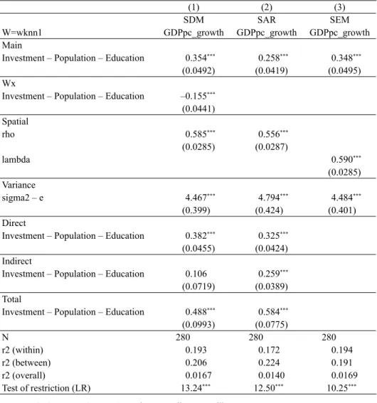
In Table 6 we further test the robustness of our results by using restricted regressions in the Ertur – Koch (2007) manner. The results indicate that the overi- dentifying restrictions are rejected.

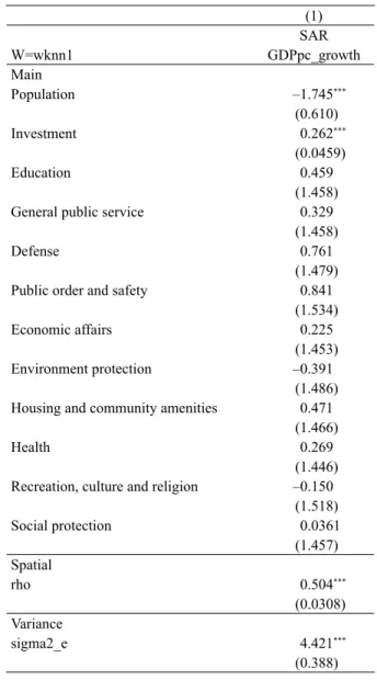
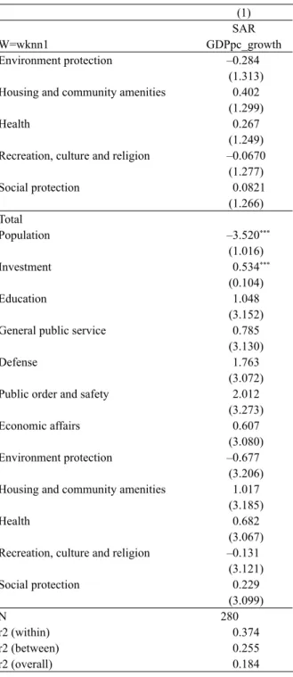
Finally, we add other government expenditures as additional control variables.

In this case, however, neither type of government expenditures is found to be statistically significant. The results are given in Table 7.

Table 7. Robustness check with other expenditure types (1) SAR

W=wknn1 GDPpc_growth

Main

Population –1.745^***

(0.610)

Investment 0.262^***

(0.0459)

Education 0.459

(1.458)

General public service 0.329

(1.458)

Defense 0.761

(1.479)

Public order and safety 0.841

(1.534)

Economic affairs 0.225

(1.453)

Environment protection –0.391

(1.486) Housing and community amenities 0.471

(1.466)

Health 0.269

(1.446) Recreation, culture and religion –0.150

(1.518)

Social protection 0.0361

(1.457) Spatial

rho 0.504^***

(0.0308) Variance

sigma2_e 4.421^***

(0.388)

(20)

(1) SAR

Direct

(0.608)

(0.0605)

Education 0.633

(1.873)

(1.858)

Defense 1.057

(1.826)

(1.947)

(1.827)

(1.889)

Health 0.414

(1.821) Recreation, culture and religion –0.0645 (1.848)

(1.837) Indirect

(0.419)

(0.0453)

Education 0.414

(1.282)

(1.276)

Defense 0.706

(1.249)

(1.329)

(1.256) Table 7. cont.

(21)

(1) SAR

(1.299)

Health 0.267

(1.277)

(1.266) Total

(1.016)

(0.104)

Education 1.048

(3.152)

(3.130)

Defense 1.763

(3.072)

(3.273)

(3.080)

(3.185)

Health 0.682

(3.121)

(3.099)

N 280

r2 (within) 0.374

r2 (between) 0.255

r2 (overall) 0.184

Note: Standard errors are in parentheses; ^* p < 0.10, ^** p < 0.05, ^*** p < 0.01.

Table 7. cont.

(22)

6. CONCLUSION

This paper analyses the impact of government expenditures on education (i.e. a productive type of government expenditures) on GDP growth in the EU28 countries during the period 2004–2013. It extends previous literature on the topic in that it uses a novel econometrics technique that allows for the spatial effects.

Namely, it is possible that GDP growth in one country depends not only on independent variables within that country but also on variables from the neighbouring countries. If this is the case, the traditional (a-spatial) econometric techniques are not appropriate, as the assumption of independent and identically distributed observations is no longer valid. In spite of the fact that the spatial econometric techniques are developing fast and gaining more importance, such approach has not been applied to the relationship between government’s education expenditures and economic growth as yet.

Studies investigating the relationship between total government size and growth typically find this relationship to be negative, leaving little scope for increasing government expenditures. From this point of view, the only solution seems to be re-structuring of the given size of the government. Theory posits that government expenditures on education have a positive impact on growth, and should, as such, be stimulated. The main goal of this paper, therefore, was to investigate whether this part of overall expenditures is indeed growth-enhancing in the EU28 countries, especially after spatial correlations among the countries in the sample are taken into account. Our results confirm this. We find that government expenditures on education significantly and positively influence GDP growth and this finding is robust in a variety of specifications. Firstly, we find that education expenditures in one country affect GDP growth in the neighbouring countries, meaning that these spillovers are geographical in nature. Moreover, we find that the degree of interdependence among the countries varies according to average GDP per capita even if geographical distances are identical. Addition- ally, immigration is found to be an important channel of spatial transmission. In each specification the indirect effects are found to be quite large, suggesting that growth models should account for the spatial interdependencies, since the omis- sion of these spillovers on neighbouring countries drastically underestimates the impact of education on growth. Indeed, Ertur – Koch (2007) also emphasise that the textbook Solow model is misspecified as it does not include these interdependencies. Therefore, countries cannot be treated as spatially independent observations; rather these spatial interactions should be accounted for explicitly.

Overall, our results suggest that investing in education is a growth-promoting activity, and it should, therefore, be supported by economic policy. Our results imply that the policy choices in one country in the EU28 generate spillover ef-

(23)

fects into other countries. These linkages are particularly important in a union of countries, such as the EU28, where individual governments might choose a level of education spending different from the optimal one from the perspective of the union as a whole. Since each government takes into account only the impact on own-country growth, supra-national policies that account for spillovers, should be brought. Precisely, since the increased education expenditures in one country increase growth in other members of the EU28, policies that account for these positive externalities should be adopted and in this way overall costs of education expenditures would be reduced.

REFERENCES

Abreu, M. – De Groot, H. – Florax, R. (2004): Space and Growth: A Survey of Empirical Evidence and Methods. Tinbergen Institute Discussion Paper, No. 04–129/3.

Acosta-Ormaechea, S. – Morozumi, A. (2013): Can a Government Enhance Long-Run Growth by Changing the Composition of Public Expenditure? IMF Working Paper, No. 13/162.

Afonso, A. – Gonzalez Alegre, J. (2008): Economic Growth and Budgetary Components. A Panel Assessment for the EU. ECB Working Paper, No. 848.

Anselin, L. – Bera, J. (1998): Spatial Dependence in Linear Regression Models with an Introduc- tion to Spatial Econometrics. In: Ullah, A. – Giles, D. (eds): Handbook of Applied Economic Statistics. New York: Marcel Dekker, pp. 237–289.

Anselin, L. – Griffi th, D. (1988): Do Spatial Effects Really Matter in Regression Analysis? Papers of the Regional Science Association, 65(1): 11–34.

Baldacci, E. – Clements, B. – Gupta, S. – Qiang, C. (2004): Social Spending, Human Capital, and Growth in Developing Countries: Implications for Achieving MDGs. IMF Working Paper, No.

04/217.

Baldacci, E. – Dell’Erba, S. – Poghosyan, T. (2011): Spatial Spillovers in Emerging Market Spreads.

IMF Working Paper, No. 11/221.

Barro, R. – Sala-i-Martin, X. (1995): Economic Growth. Cambridge: MIT Press.

Benhabib, J. – Spiegl, M. (1994): The Role of Human Capital in Economic Development: Evidence from Aggregate Cross-Country Data. Journal of Monetary Economics, 34(2): 143–173.

Bose, N. – Haque, E. – Osborn, D. (2007): Public Expenditure and Economic Growth: A Disaggre- gated Analysis for Developing Countries. The Manchester School, 75(5): 533–556.

Colombier, C. (2011): Does the Composition of Public Expenditure Affect Economic Growth?

Evidence from the Swiss Case. Applied Economics Letters, 18(16): 1583–1589.

Cravo, T. – Becker, B. – Gourlay, A. (2015): Regional Growth and SMEs in Brazil: A Spatial Panel Approach. Regional Studies, 49(12): 1995–2016.

Elhorst, P. (2014): Spatial Econometrics. From Cross-Sectional Data to Spatial Panels. London:

Springer.

Ertur, C. – Koch, W. (2007): Growth, Technological Interdependence and Spatial Externalities:

Theory and Evidence. Journal of Applied Econometrics, 22(6): 1033–1062.

European Commission (2010): Europe 2020 – A European Strategy for Smart, Sustainable and Inclusive Growth. http://ec.europa.eu/eu2020/pdf/

Eurostat (2016): Government Finance and EDP Statistics Database. http://ec.europa.eu/eurostat/

web/government-fi nance-statistics/data/database.