Comparison of Various Data Mining Classification Techniques in the Diagnosis of Diabetic Retinopathy

Comparison of Various Data Mining

Classification Techniques in the Diagnosis of Diabetic Retinopathy

Spandana Vadloori

, Yo-Ping Huang

and Wei-Chi Wu

1Department of Electrical Engineering, National Taipei University of Technology, Taipei, Taiwan 10608; yphuang@ntut.edu.tw

2Department of Computer Science and Information Engineering, National Taipei University, New Taipei City, Taiwan 23741

3Department of Ophthalmology, Chang Gung Memorial Hospital, Linkou, Taoyuan, Taiwan 33333

4College of Medicine, Chang Gung University, Taoyuan, Taiwan 33333

*Corresponding author

Abstract: Diabetic retinopathy (DR) has been the most frequently occurring complication in the patients suffering from a long-term diabetic condition, that ultimately leads to blindness. Early detection of the disease through biomarkers and effective treatment has been proposed to prevent/delay its occurrence. Several biomarkers have been explored, to help understand the incidence and progression of DR. These included the presence of microaneurysms, exudates, hemorrhages, etc. in the retina of the patients, which contributes to the disease. Investigation of the retinal images from time to time has been proposed as a strategy to prevent blindness. Evaluating the retinal images manually is time-consuming and demands great expertise in the diagnosis of DR. To circumvent such issues computer-aided diagnosis are very promising in the detection of DR. In the present study, we used a DR dataset and applied different classification algorithms in machine learning to predict the occurrence of the DR. The classifiers employed herein, included K- nearest neighbor, random forest classifier, support vector machine, regression tree classifier, logistic regression and the Naïve Bayes theorem. Our results showed that the random forest classification model provided the significant detail of attributes in terms of their importance in the diagnosis of the DR. More importantly, our supervised classification models provided the prediction accuracy of the disease and Naïve Bayes classifier demonstrated highest accuracy of 80.15% in the prediction of DR compared to the others. Additionally, receiver operating characteristics (ROC) analysis, with the classifiers and the area under curve (AUC) represented the fitting results of each classifier.

The presented approach can prove to be a potential tool for the ophthalmologist in the early diagnosis tool for DR.

Keywords: diabetic retinopathy (DR); data mining; retinal images; microaneurysms;

exudates; classification

1 Introduction

Diabetic Retinopathy (DR) is the most common, yet a serious condition that occurs in patients who are suffering from chronic, severe diabetes and may lead to damaged retinas, causing blindness if not diagnosed and treated in the early stages [1-3]. DR is commonly observed in 80% of the individuals who are suffering due to diabetes for more than 20 years [1]. Statistics reveal that the occurrence of DR is increasing at an alarming rate, and as stated by WHO (World Health Organization), DR reports for 4.8% of the 37 million cases of blindness that take place globally [4]. By 2030 more than 366 million people are estimated to suffer from DR [2].

DR is a progressive disease that develops gradually. The development of DR has been grouped into four stages, (1) mild-NPDR (non-proliferative diabetic retinopathy), (2) moderate-NPDR, (3) severe-NPDR and (4) proliferative diabetic retinopathy (PDR) [5, 6]. Mild-NPDR is the early stage of DR characterized by the swelling of the retinal blood vessels. These balloon-like swollen blood vessels appear as dark red dots called microaneurysms (MAs) whose sizes range from 20 to 200 microns [7, 8]. Leakage of MAs is a noticeable and essential sign for the detection of DR. In the second stage of DR, known as moderate-NPDR, the retinal blood vessels swell and get blocked that leads to a state called diabetic macular edema (DME). This fluid further increases in the macular zone of the retina leading to the third stage called severe-NPDR where the DR symptoms become worse. Initially mild-, moderate- and severe-NPDR were classified as three different groups. However, later they were combined into a single group called NPDR. The final stage of the DR is called PDR, where more blood vessels are generated inside the retina and a fluid called vitreous gel is filled in the eyes. Such blood vessels are very fragile and prone to fluid leakage and bleeding consequently forming a scar tissue that leads to the retinal detachment. In addition to MAs, the other biomarkers for DR are exudates (EXU). These exudates are round or oval-shaped fatty protein-based particles found in the nerve fiber layers of the retina that are formed in the NPDR state due to fluid leakage from the damaged retinal blood vessels and had been linked to blindness [9]. Depending on their appearance EXUs were divided into two types, hard EXUs and soft EXUs, which appear as the hard waxy patches and softer EXUs respectively. These soft EXUs are also called cotton wool EXUs (Figure 1). Hard EXUs are located near MAs or at the edges of the retinal edema. Regular screening of the retinal images in diabetic patients has been proposed for early diagnosis of the DR diseases, which can prevent people from becoming blind [10, 11].

Data mining is a process of analyzing the raw information from a large information database and turning it into useful information where meaningful patterns and trends of the data emerge [12]. Data mining has been potentially useful in various areas of healthcare [13, 14]. Today, the healthcare industry produces copious data about patients, clinical symptoms, disease detection techniques, etc. Extracting healthcare data could be very useful to perform medicinal evaluations to diagnose or cure disease. Particularly data mining has gained momentum in identifying the risk of cardio-vascular diseases [15, 16], lung diseases [17], cancer [18], diabetes [19], etc.

Figure 1

Comparison of the retinal images from (A) normal and (B) with the lesion of NPDR In the present study, we focused on evaluation of the DR dataset by using various data mining classification techniques. This strategy enabled us to determine the prediction accuracy of the DR. We further evaluated the performance of the classifier models by calculating the sensitivity and specificity of these models.

Our results showed that the Naïve Bayes classifier was the most efficient classification model compared to the others and also addressed the significant contribution of attributes in the diagnosis of DR.

This paper has been organized as follows. Dataset used to test different classifiers were introduced in Section 2. Test results and discussions were presented in Section 3. The conclusions and future work were given in Section 4.

2 Detailed Attributes of Dataset

In the present study, we tested the Diabetic Retinopathy Debrecen (DRD) dataset accessible from UCI Machine Learning Repository [20]. The dataset comprised of the attribute features extracted from Messidor images. In light of this dataset, we anticipated whether the image has indications of having DR or no DR. Based on Hidden Markov Random fields (HMRF) [21] the quality of the images in the dataset was assessed. The retinal images were characterized during the initial pre- screening step and all the attributes features were extracted [22]. This information was accessible from the dataset and we performed analysis on this dataset. But the problem is that there is no report, on which those attributes, that are critical for the annotation of patients with DR are available. The detailed features and attributes in the dataset and image description are given in Table 1 and Table 2, respectively.

Table 1

Details of the featured indices of the dataset Dataset characteristics Number of instances 1151 Attribute characteristics Integer, Float Number of attributes 20

Associated tasks Classification Table 2

Dataset attributes and their descriptions

Attribute Description

1 Binary result of quality assessment 0: bad

1: sufficient quality

2 Binary result of pre-screening 0: Lack of retinal abnormality 1: presence of retinal abnormality

3-8 Results of Micro aneurysm detection revealing the number of Micro aneurysms at varying confidence levels alpha =0.5 to 1

9-16 The exudates contained the same information as microaneurysms (3-8), where they are represented by a set of points instead of number of pixels constructing the lesions. These features were normalized by dividing the number of lesions with the diameter of the ROI to compensate different image sizes

17 Euclidean distance between the center of the macula and the center of the optic disc

18 Optic disk diameter

19 The binary result of AM/FM classification 20 Presence or absence of DR

1: Presence of DR (accumulation of 1,2,3 stages in Messidor) 0: Healthy

MAs were identified by preprocessing method and candidate extractor ensembles [23], while EXUs were detected by optimal combinations of ensemble-based system through voting system [24]. They did not mention among the candidate factors which MAs and EXUs were critical in determining DR. In this study, the dataset containing 1151 samples was cleaned by removing bad quality samples from the dataset. Furthermore, we also preprocessed for outliers using Python program by setting a threshold to 3. The final dataset contained 983 samples, which were later divided into 60% for training and 40% for prediction dataset.

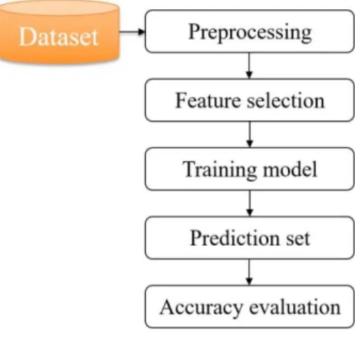
Figure 2 illustrates the framework of the methodology used.

Figure 2

Framework for classification methodology

The performance of all these models was evaluated by calculating the sensitivity, specificity and accuracy based on the formulas given below:

%

100

 

FN TP y TP

Sensitivit (1)

%

100

 

TN FP y TN

Specificit (2)

%

100







 

FN TN FP TP

TN

Accuracy TP (3)

where TP: true positive; TN: true negative, FN: false negative, FP: false positive.

Additionally, we performed Area Under the Curve (AUC) and Receiver Operating Characteristics (ROC) curve to display the performance of the models. In AUC, the value always lies between 0 and 1 [25]. This is useful to visualize the classification problems to distinguish between the classes.

3 Results and Discussions

In this study, we analyzed a total of 983 samples from the dataset. This dataset included 51.3% of patients diagnosed with DR (indicated by 1), while the remaining 48.7% were not diagnosed with DR (indicated by 0). Attributes with higher variance were proposed to have valuable information [26]; therefore, we performed attribute scores (Table 3) and removed the low-scoring attributes which were almost zero, namely EC.DIST. and OPT.DIA.

The dataset was characterized by using various classifiers with a motivation to predict the occurrence of DR, derive the rules in diagnosis of DR and understand the importance of attributes in detection of the DR. Six classification models were evaluated for the disease prediction accuracy, which included K-NN, random forest, regression tree, SVM, logistic regression, and Naïve Bayes. All the experiments were carried out in XLSTAT.

Initially, the classification model was trained and the prediction results from the test dataset were analyzed by the classifier using the DR attributes, MAs and EXUs, etc. The prediction accuracy of each classifier model was evaluated based on the result that determines the presence or absence of the disease. Later, we evaluated all the classification models tested in the study, and compared the accuracy of each of the models in detection of DR. The attributes and their statistical representations are given in Table 3.

Table 3

Summary statistics (training/quantitative) of the dataset

Attribute Minimum Maximum Mean Std. deviation Score

MAœ=0.5 1.00 151.00 38.43 25.62 0.47

MAœ=0.6 1.00 132.00 36.91 24.11 2.91

MAœ=0.7 1.00 120.00 35.14 22.81 14.02

MAœ=0.8 1.00 105.00 32.30 21.11 38.75

MAœ=0.9 1.00 97.00 28.75 19.51 60.79

MAœ=1.0 1.00 89.00 21.15 15.10 66.31

EXU1 0.35 403.90 64.10 58.49 4.60

EXU2 0.00 167.10 23.09 21.60 29.69

EXU3 0.00 106.10 8.71 11.57 18.88

EXU4 0.00 59.77 1.84 3.92 1.03

EXU5 0.00 51.42 0.56 2.48 37.38

EXU6 0.00 20.10 0.21 1.06 23.40

EXU7 0.00 5.94 0.09 0.40 16.46

EXU8 0.00 3.09 0.04 0.18 7.36

EC. DIST. 0.37 0.59 0.52 0.03 0.00

OPT.DIA. 0.06 0.22 0.11 0.02 0.00

AM/FM 0.00 1.00 0.34 0.47 0.13

In K-NN classification, the class of the query is obtained based on the nearest neighbors to that of the example query. K-NN searches the pattern to the closest data and then assigns to data that is unknown [27]. In this classification, we used Euclidean distance as a criterion along with 10-fold cross validation to predict the class label from the prediction dataset. With K-NN classification system, 71.25%

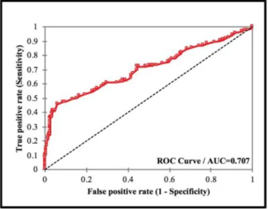
of accuracy was achieved from the prediction dataset as shown in Table 4. The results based on prediction class showed 205 samples without DR, while 188 samples showed the occurrence of DR. The results were given in Table 5, where the first 10 predicted results in each class were shown as representation for all the test cases from the dataset. Here, the terminology PredObs indicates with the sample number from the prediction dataset. For example, PredObs1 means that the 1^st out of 393 patients was predicted to be no DR. Similarly, PredObs7 indicates that the 7^th patient was predicted to have DR. In K-NN, we obtained AUC value of 0.707 (Figure 3).

Table 4 K-NN based classification Confusion matrix (prediction dataset)

from \ to 0 1 Total %

0 146 54 200 73.00

1 59 134 193 69.43

Total 205 188 393 71.25

Table 5

K-NN prediction results by class

Class 0 1

Objects 205 188

PredObs1 PredObs7 PredObs2 PredObs10 PredObs3 PredObs11 PredObs4 PredObs14 PredObs5 PredObs16 PredObs6 PredObs17 PredObs8 PredObs19 PredObs9 PredObs28 PredObs12 PredObs30 PredObs13 PredObs32

Figure 3 ROC for K-NN model

The next classification system we tested was random forest. In this type of classification, many small decision-trees are merged into a forest that displays the classification table of well-classified observations. Usually this classifier is fast and robust to noise and has better explanation and visualization of its output [28]. This classifier does eliminate the possibility of overfitting the data.

Importantly, random forest classifier in our study has identified the most important attributes from the training dataset. Here, we used bagging approach to obtain more accurate results. We observed MAs and EXUs were two critical attributes in detecting DR. Among all the MAs, MA0.5 was seen as a critical attribute. In the case of EXUs, EXU7 was critical followed by EXU1 (Figure 4).

In this classification model an accuracy of 72.71% (Table 6) was achieved in the training set and 71.76% with the prediction set. Here, we obtained AUC value of 0.715 (Figure 5).

Table 6

Accuracy as determined by using random forest classifier Confusion matrix –Training set

From \ to 0 1 Total Accuracy (%)

0 210 88 298 70.47

1 73 219 292 75.00

Total 283 307 590 72.71 Confusion matrix –Prediction set From \ to 0 1 Total Accuracy (%)

0 147 49 196 75.00

1 62 135 197 68.53

Total 209 184 393 71.76

Figure 4

Significance of attributes classified by random forest classifier

We also tested the classification by the regression tree method. This classifier uses the trained dataset and generates itself correctly in order to generate a decision tree. Such decision trees are quite easy to understand and analyze. In this model the decisions are predicted by following the decisions from the root node and to the leaf node. The response of occurrence of the DR is present in the leaf node.

Depending on the working process of learning, any new input data would be classified in generation of decision tree [29].

Figure 5

ROC for random forest model

This classification system also generated the rules with the critical attribute relating to the possibility of occurrence of DR (Table 7). The rules predict the number of cases with and without DR, based on the individual attributes and also

the combination of different attributes. These rules show 80% of the cases were without DR when the attribute EXU7 ≤ 0.01029 and 10% of the case were with DR when the EXU7  0.136501. 27.1% of the cases are with no DR when the EXU7  0.01029 and MAα=0.5  18. 7.8% of the cases are no DR when the EXU7  0.01029 and the value of MAα=0.5  18. 17.5% of the cases are with DR when the value of the EXU7  0.01029 and the value of the MAα=0.5 is between 18 and 38. 14.7% of the cases are with DR when the value of EXU7  0.01029 and MAα=0.5 is between 46 and 61, etc. (Table 8). Moreover, this system also evaluates the most possible prediction using the combination of the attributes.

This process involves several dimensions including splitting criterion, stopping rules, branch condition, etc. In this study, an accuracy of 72.71% on training dataset and 72.77% on the prediction dataset was achieved (Table 8) in classifying the occurrence/non-occurrence of DR. By this model AUC of 0.749 was obtained (Figure 6).

Table 7

Rules of the attributes generated by regression tree classifier in diagnosis of DR DR

(Pred) Rules

0 If EXU7  0.01029 then CLASS LABEL = 0 in 80% of cases

1 If EXU7 (0.01029, 0.136501] then CLASS LABEL = 1 in 10% of cases 1 If EXU7 > 0.136501 then CLASS LABEL = 1 in 10% of cases 0

If EXU7  0.01029 and MAœ=0.5  18 then CLASS LABEL = 0 in 27.1% of cases

1

If EXU7  0.01029 and MAœ=0.5 (18, 38] then CLASS LABEL = 1 in 17.5% of cases

0

If EXU7  0.01029 and MAœ=0.5 (38, 46] then CLASS LABEL = 0 in 7.8% of cases

1

If EXU7  0.01029 and MAœ=0.5 (46, 61] then CLASS LABEL = 1 in 14.7% of cases

1

If EXU7 (0.01029, 0.136501] and EXU3  9.74204 then CLASS LABEL

= 1 in 6.3% of cases 0

If EXU7 (0.01029, 0.136501] and EXU3 (9.74204, 19.4151] then CLASS LABEL = 0 in 2.0% of cases

1

If EXU7 (0.01029, 0.136501] and EXU3 > 19.4151 then CLASS LABEL

= 1 in 1.7% of cases 0

If EXU7 > 0.136501 and EXU5  0.275714 then CLASS LABEL = 0 in 0.3% of cases

1

If EXU7 > 0.136501 and EXU5 > 0.275714 then CLASS LABEL = 1 in 9.7% of cases

1

If EXU7  0.01029 and MAœ=0.5 (18, 38] and MAœ=0.7 MAœ=0.8  16 then CLASS LABEL = 1 in 1.2% of cases

0

If EXU7  0.01029 and MAœ=0.5 (18, 38] and MAœ=0.7 MAœ=0.8 >

16 then CLASS LABEL = 0 in 16.3% of cases

1

If EXU7  0.01029 and MAœ=0.5 (38, 46] and MAœ=0.9  35 then CLASS LABEL = 1 in 2.7% of cases

0

If EXU7  0.01029 and MAœ=0.5 (38, 46] and MAœ=0.9 > 35 then CLASS LABEL = 0 in 5.1% of cases

1

If EXU7  0.01029 and MAœ=0.5 (46, 61] and EXU4  0.747636 then CLASS LABEL = 1 in 8.8% of cases

0

If EXU7  0.01029 and MAœ=0.5 (46, 61] and EXU4 > 0.747636 then CLASS LABEL = 0 in 5.9% of cases

1

If EXU7  0.01029 and MAœ=0.5 > 61 and EXU1  34.5626 then CLASS LABEL = 1 in 7.6% of cases

0

If EXU7  0.01029 and MAœ=0.5 > 61 and EXU1 (34.5626, 66.7516]

then CLASS LABEL = 0 in 4.6% of cases 1

If EXU7  0.01029 and MAœ=0.5 > 61 and EXU1 > 66.7516 then CLASS LABEL = 1 in 0.7% of cases

1

If EXU7 (0.01029, 0.136501] and EXU3  9.74204 and MAœ=0.9  41 then CLASS LABLE = 1 in 3.4% of cases

0

If EXU7 (0.01029, 0.136501] and EXU3  9.74204 and MAœ=0.9 (41, 45] then CLASS LABEL = 0 in 0.7% of cases

1

If EXU7 (0.01029, 0.136501] and EXU3  9.74204 and MAœ=0.9 > 45 then CLASS LABLE = 1 in 2.2% of cases

0

If EXU7 (0.01029, 0.136501] and EXU3 (9.74204, 19.4151] and OPTDIA  0.089971 then CLASS LABEL = 0 in 0.5% of cases

1

If EXU7 (0.01029, 0.136501] and EXU3 (9.74204, 19.4151] and OPTDIA (0.089971, 0.100454] then CLASS LABEL = 1 in 0.3% of cases

0

If EXU7 (0.01029, 0.136501] and EXU3 (9.74204, 19.4151] and OPTDIA > 0.100454 then CLASS LABEL = 0 in 1.2% of cases 1

If EXU7  0.01029 and MAœ=0.5 > 61 then CLASS LABEL = 1 in 12.9% of cases

Table 8

Classification of dataset based on regression tree Confusion matrix –Training set From \ to 0 1 Total Accuracy (%)

0 241 38 279 86.38

1 123 188 311 60.45

Total 364 226 590 72.71 Confusion matrix –Prediction set From \ to 0 1 Total Accuracy (%)

0 159 66 225 70.67

1 41 127 168 75.60

Total 200 193 393 72.77

Figure 6

ROC for regression tree model

Next, we performed SVM classification, which is a supervised learning method and belongs to family of linear classification. It is one of the powerful methods in classification where a decision boundary is created through which the class labels are predicted from the feature vectors. SVM is good at recognizing patterns in complex datasets. However, there is no particular “best” kernel to recognize the patterns. The only way to select the best kernel is by trial and error [30]. We used linear Kernel and preprocessed by rescaling. We performed data validation using 150 samples for better fitting of the model since the model resulted in over-fitting.

In this model, we obtained the accuracy of 74.32% on training set, 70.23% on prediction set (Table 9) and 64.67% on validation set. Performance metrics from this classifier indicated the sensitivity (recall) and specificity (Table 10). AUC was 0.809 with SVM model (Figure 7).

Table 9

Classification of dataset based on SVM Confusion matrix –Training set From \ to 0 1 Total Accuracy (%)

0 201 27 228 88.16

1 86 126 212 59.43

Total 287 153 440 74.32 Confusion matrix –Validation set From \ to 0 1 Total Accuracy (%)

0 55 7 62 88.71

1 46 42 88 47.73

Total 101 49 150 64.67

Confusion matrix –Prediction set From \ to 0 1 Total Accuracy (%)

0 170 19 189 89.95

1 98 106 204 51.96 Total 268 125 393 70.23

Table 10

Performance metrics (Class label of DR 0 / 1) Statistic Training set (%) Validation set (%)

Accuracy 0.743 0.647

Precision 0.700 0.545

Recall 0.882 0.887

F-score 0.781 0.675

Specificity 0.286 0.280

FPR 0.714 0.720

Prevalence 0.457 0.367

NER 0.518 0.413

Figure 7

ROC for support vector machine

Logistic regression, a machine learning algorithm and a kind of linear regression classification model, for predictive analysis based on probability that depends on the linear measurement of the samples. It is the most commonly used statistical classification when the dependent variable is dichotomous, i.e., either positive or negative. This regression model inspects the bond between the independent and dependent variables of binary outcome and is extensively used in applications like medical and biomedical research, to predict the outcome. The logistic regression equation was used to estimate the possibility of specified consequence [31]. In the present study, we found that the logistic regression showed an accuracy of 74.41%

for training set and 73.28% for the prediction set (Table 11). Here, we obtained AUC value of 0.764 (Figure 8), signifying 76.4% of the chance this model can distinguish correctly between those with or without DR. Our results show a higher AUC representing good performance of the model.

Table 11

Accuracy from logistic regression classification Confusion matrix –Training set From \ to 0 1 Total Accuracy (%)

0 234 49 283 82.69

1 102 205 307 66.78

Total 336 254 590 74.41

Confusion matrix –Prediction set From \ to 0 1 Total Accuracy (%)

0 164 32 196 83.67

1 73 124 197 62.94

Total 237 156 393 73.28

Figure 8

ROC for logistic regression model

Finally, we examined Naïve Bayes classification model for analyzing the dataset.

Naïve Bayes is a supervised machine learning algorithm that classifies the observations based on the instructions set by the algorithm itself. Naïve Bayes is one of the efficient and effective classifier that works on the principle of Bayes theorem. Naïve Bayes has proven to be robust and simple probabilistic and was known for its best performance in the classification of medical data [32].

Compared to other classifiers this classification was found to be more effective computationally, where a small training dataset is sufficient enough for more accurate prediction of disease [33]. It was also reported to diagnose the disease just like a physician, considering the available attributes for the prediction analysis [34]. In this classification, the system was initially trained with the set of inputs from the training dataset that were further refined and classified for the prediction dataset. Here, we used 10-fold cross validation to predict the classes from the prediction dataset. Therefore, in the present study, 590 cases were considered as training dataset (Table 12) and the remaining cases were taken as test dataset.

Based on this classification system, the class label results predicted 212 cases without DR, while 181 cases were with DR. The first 10 predicted results in each class were shown as representation for all the test cases from the dataset (Table 13). In this study, Naïve Bayes method showed 83.56% of accuracy on training set and 80.15% of accuracy on prediction set in determining the occurrence of DR.

Here, we obtained AUC value of 0.816 (Figure 9). When comparing the results shown in Table 13 to Table 5, we found some inconsistencies from the classifications. For example, PredObs1 and PredObs3 were classified to Class 0 by K-NN but were group to Class 1 by Naïve Bayes classifier. By contrast, PredObs2 was classified to Class 0 by both classifiers.

Table 12

Naïve Bayes classification on training set Confusion matrix –Training set

From \ to 0 1 Total Accuracy (%)

0 257 22 279 92.11

1 75 236 311 75.88

Total 332 258 590 83.56

Confusion matrix – Prediction set

From \ to 0 1 Total Accuracy (%)

0 167 33 200 83.50

1 45 148 193 76.68

Total 212 181 393 80.15

Table 13

Prediction accuracy from Naïve Bayes classification on test dataset

Class 0 1

Objects 212 181

PredObs2 PredObs1 PredObs4 PredObs3 PredObs5 PredObs9 PredObs6 PredObs10 PredObs7 PredObs11 PredObs8 PredObs13 PredObs12 PredObs14 PredObs15 PredObs18 PredObs16 PredObs25 PredObs17 PredObs28

Figure 9 ROC for Naïve Bayes model

Among all the six classifiers that were studied thoroughly in the current study, our results suggested that the Naïve Bayes model of classification displayed the best accuracy followed by logistic regression model (Table 14).

Table 14

Accuracy achieved by different classification models No. Classification model Accuracy (%)

1 K-NN 71.25

2 Random forest 71.76 3 Regression tree 72.77

4 SVM 70.23

5 Logistic regression 73.28

6 Naïve Bayes 80.15

Conclusions

Diabetic retinopathy is the main cause of blindness for patients suffering from diabetes mellitus. In spite of the fact that early identification of retinal images for the disease symptoms have been proposed and could prevent or delay its occurrence, the approach falls short, due to the limited availability of human expertise and lack of infrastructure to detect DR manually. Nevertheless, data mining serves as an essential tool to carry out classification and diagnose the disease. In the present study, we assessed the Messidor DR dataset, employed various classification models and evaluated their prediction accuracy in diagnosis of DR. We determined the significant role of attributes individually and in combination with other attributes crucial in the development of DR. Naïve Bayes performed best, among the six classifiers, in terms of accuracy and performance in evaluation.

In the future, we aim to develop deep learning algorithms to automatically pre- screen images for the diagnosis of DR.

Acknowledgement

This study was funded in part by the Ministry of Science and Technology, Taiwan, under Grants MOST107-2221-E-027-113- and MOST108-2321-B-027- 001-. and by a joint project between the National Taipei University of Technology and the Chang Gung Memorial Hospital under Grant NTUT-CGMH-106-05.

References

[1] M. M. Nentwich and M. W. Ulbig: Diabetic retinopathy-ocular complications of diabetes mellitus, World Journal of Diabetes, Vol. 6, No.

3, Apr 2015, pp. 489-499

[2] Y. Zheng, M. He and N. Congdon: The worldwide epidemic of diabetic retinopathy, Indian Journal Ophthalmology, Vol. 60, Sep-Oct 2012, pp.

428-431

[3] S. K. Lynch and M. D. Abramoff: Diabetic retinopathy is a neurodegenerative disorder, Vision Research, Vol. 139, Oct 2017, pp. 101- 107

[4] J. L. Leasher, R. R. A. Bourne, S. R. Flaxman, J. B. Jonas, J. Keeffe, N.

Naidoo, K. Pesudovs, H. Prince, R. A. White, T. Y. Wong, S. Resnikoff and H. R. Taylor: Global estimates on the number of people blind or visually impaired by diabetic retinopathy: a meta-analysis from 1990-2010, Diabetes Care, Vol. 39, Nov 2016, pp. 2096-2096

[5] K. C. Jordan, M. Menolotto, N. M. Bolster, I. A. T. Livingstone and M. E.

Giardini: A review of feature-based retinal image analysis, Expert Review of Ophthalmology, Vol. 12, No. 3, Mar 2018, pp. 207-220

[6] J. Amin, M. Sharif and M. Yasmin: A review on recent developments for detection of diabetic retinopathy, Scientifica, Vol. 2016, May 2016, pp. 1- 20

[7] M. Dubow, A. Pinhas, N. Shah, R. F. Cooper, A. Gan, R. C. Gentile, V.

Hendrix, Y. N. Sulai, J. Carroll, T. Y. Chui, J. B. Walsh, R, Weitz, A.

Dubra and R. B. Rosen: Classification of human retinal microaneurysms using adaptive optics scanning light ophthalmoscope fluorescein angiography, Investigative Ophthalmology and Visual Science, Vol. 55, Mar 2014, pp. 1299-1309

[8] L. Dai, R. Fang, H. Li, X. Hou, B. Sheng, Q. Wu and W. Jia: Clinical report guided retinal microaneurysm detection with multi-sieving deep learning, IEEE Trans. on Medical Imaging, Vol. 37, No. 5, Jan 2018, pp. 1149-1161 [9] E. M. Kohner, I. M. Stratton, S. J. Aldington, R. C. Turner and D. R.

Matthews: Microaneurysms in the development of diabetic retinopathy (UKPDS 42), Diabetologia, Vol. 42, issue 9, Sep 1999, pp. 1107-1112

[10] M. V. Jimenez-Baez, H. Marquez-Gonzalez, R. Barcenas-Contreras, C.

Morales-Montoya and L. F. Espinosa-Garcia: Early diagnosis of diabetic retinopathy in primary care, Colombia Medica, Vol. 46, Jan-Mar 2015, pp.

14-18

[11] B. Corcostegui, S. Duran, M. O. Gonzalez-Albarran, C. Hernandez, J. M.

Ruiz-Moreno, J. Salvador, P. Udaondo and R. Simo: Update on diagnosis and treatment of diabetic retinopathy: a consensus guideline of the working group of ocular health (Spanish Society of Diabetes and Spanish Vitreous and Retina Society), Journal of Ophthalmology, Vol. 2017, Jun 2014, p. 10 [12] A. K. Pujari: Data Mining Techniques, Universities Press, India, Feb 2001,

p. 44

[13] M. Ilayaraja and T. Meyyappan: Mining medical data to identify frequent diseases using Apriori algorithm, in proc. of Int. Conf. on IEEE Int. Symp.

on Pattern Recognition, Informatics and Mobile Engineering, Salem, Apr 2013, pp. 194-199

[14] J. C. Prather, D. F. Lobach, L. K. Goodwin, J. W. Hales, M. L. Hage, and W. E. Hammond: Medical data mining: knowledge discovery in a clinical data warehouse, in proc. of Int. Conf. AMIA Annu Fall Symp. 1997, pp.

101-105

[15] T.-H. Cheng, C.-P. Wei and V. S. Tseng: Feature selection for medical data mining: Comparisons of expert judgment and automatic approaches, in Proc. of Int. Conf. on 19^th IEEE Int. Symp. on Computer-Based Medical Systems, Salt Lake City, UT, 2006, pp. 165-170

[16] W. Xue, Y. Sun and Y. Lu: Research and application of data mining in traditional Chinese medical clinic diagnosis, in Proc. of Int. Conf. on IEEE Int. Symp. On Signal Processing, Beijing, 2006, pp. 1-4

[17] S. M. Khan, R. Islam and M. U. Chowdhury: Medical image classification using an efficient data mining technique, on Proc. of Int. Conf. on Machine Learning and Applications, Louisville, Kentucky, USA, 2004, pp. 397-402 [18] P.-H. Tang and M. Tseng: Medical data mining using BGA and RGA for

weighting of features in fuzzy k-NN classification, in Proc. of Int. Conf. on Machine Learning and Cybernetics, Hebei, 2009, pp. 3070-3075

[19] S. Balakrishnan, R. Narayanaswamy, N. Savarimuthu and R. Samikannu:

SVM ranking with backward search for feature selection in type II diabetes databases, in Proc. of Int. Conf. on IEEE Int. on Systems, Man and Cybernetics, Singapore, 2008, pp. 2628-2633

[20] UCI, Diabetic Retinopathy Debrecen dataset, [Online].

Available:https://archive.ics.uci.edu/ml/datasets/Diabetic+Retinopathy+De brecen+Data+Set, Accessed on. Sep 2018

[21] G. Kovács and A. Hajdu: Extraction of vascular system in retina images using averaged one-dependence estimators and orientation estimation in hidden Markov random fields, in Proc. of Int. Conf. on IEEE Int. Symp. on Biomedical Imaging: From Nano to Macro, Chicago, IL, USA, Mar-Apr 2011, pp. 693-696

[22] B. Antal, A. Hajdu, Z. Maros-Szabo, Z. Torok, A. Csutak and T. Peto: A two-phase decision support framework for the automatic screening of digital fundus images, Journal of Computational Science, Vol. 3, Sep 2012, pp. 262-268

[23] B. Antal and A. Hajdu: An ensemble-based system for microaneurysm detection and diabetic retinopathy grading, IEEE Trans. on Biomedical Engineering, Vol. 59, No. 6, Jun 2012, pp. 1720-1726

[24] B. Nagy, B. Harangi, B. Antal and A. Hajdu: Ensemble-based exudate detection in color fundus images, in Proc. of Int. Conf. on 7^th Int. Symp. on Image and Signal Processing and Analysis, Dubrovnik, Croatia, Sep 2011, pp. 700-703

[25] T. Fawcett: An introduction to ROC analysis, Pattern Recognition Letters, Vol. 27, Jun 2006, pp. 861-874

[26] A. Yousefpour, H. N. A. Hamed, U. H. H. Zaki, K. A. M. Khaidzir: Feature subset selection using mutual standard deviation in sentiment mining, in Proc. of Int. conf. on IEEE Int. on Big Data and Analytics, Kuching, Malaysia, Nov 2017, pp. 13-18

[27] P. Rani: A review of various KNN techniques, International Journal for Research in Applied Science & Engineering Technology, Vol. 5, Aug 2017, pp. 1174-1179

[28] E. Goel and E. Abhilasha: Random forest: A review, International Journal of Advanced Research in Computer Science and Software Engineering, India, Vol. 7, Jan 2017, pp. 251-251

[29] K. A. Kaur and L. Bhutani: A Review on Classification Using Decision Tree, International Journal of Computing and Technology, Vol. 2, Feb 2015, pp. 42-46

[30] S. Huang, N. Cai, P. P. Pacheco, S. Narandes, Y. Wang and W. Xu:

Applications of support vector machine (SVM) learning in cancer genomics, Cancer Genomics & Proteomics, Canada, 2018, pp. 41-51 [31] S. R. N. Kalhori, M. Nasehi, X.-J. Zeng: A logistic regression model to

predict high risk patients to fail in tuberculosis treatment course completion, IAENG International Journal of Applied Mathematics, Vol. 40, No. 2, May 2010

[32] I. Rish: An empirical study of the naïve bayes classifier, in Proc. of Int.

Conf. on International Joint Conferences on Artificial Intelligence, Watson Research Center, Hawthorne, Jan 2001, pp. 41-46

[33] K. M. Al-Aidaroos, A. A. Bakar and Z. Othman: Naïve Bayes variants in classification learning, in Proc. of Int. Conf. on IEEE Int. on Information Retrieval & Knowledge Management, Shah Alam, Selangor, May 2010, pp.

276-281

[34] K. M. A1-Aidaroos, A. A. Bakar and Z. Othman: Medical data classification with Naïve Bayes approach, Information Technology Journal, Vol. 11, No. 9, 2012, pp. 1166-1174