Functional Genomic Annotation of Genetic Risk Loci in Chronic Kidney Disease
Ph.D. Thesis
Nóra Ledó, M.D.
Doctoral School of Basic Medicine Semmelweis University
Consultants: Katalin Suszták, M.D., Ph.D.
András Tislér, M.D., Ph.D.
Official reviewers: Tamás Szelestei, M.D., Ph.D.
Kálmán Tory, M.D., Ph.D.
Head of the Complex Examination Committee:
Péter Nyirády, M.D., D.Sc.
Members of the Complex Examination Committee:
Ágnes Haris, M.D., Ph.D.
László Wagner, M.D., Ph.D.
Budapest
2017
2
1. Table of Contents
1. Table of Contents ... 2
2. Abbreviations ... 4
3. Introduction ... 7
3.1. Chronic kidney disease, as a gene environmental disease ... 7
3.2. Different genetic methods for understanding CKD development ... 8
3.2.1. Genome-wide association studies (GWAS) ... 8
3.2.2. Expression quantitative trait loci analysis (eQTL) ... 9
3.2.3. Functional genomics ... 11
3.2.4. Other methods of CKD research ... 14
4. Objectives ... 16
5. Methods ... 17
5.1. Human kidney samples ... 17
5.1.1. Tissue handling and microdissection ... 17
5.1.2. Sample characteristics ... 17
5.2. Sample processing and data analysis ... 24
5.2.1. Microarray process and data analysis ... 24
5.2.2. RNA sequencing analysis ... 25
5.2.3. Quantitative real time polymerase chain reaction (QRT-PCR) analysis... 25
5.2.4. Genotyping of human kidney samples ... 25
5.2.5. Histology ... 26
5.3. Bioinformatics ... 26
5.3.1. Gene ontology and network analyses ... 26
5.3.2. Processing publicly available datasets ... 26
5.4. Overview of the used statistical methods... 27
3
6. Results ... 28
6.1. Identifying CKD risk associated transcripts (CRATs) ... 28
6.2. Kidney-specific expression of CRATs ... 35
6.3. Expression profile of CRATs in normal and disease human kidney samples ... 37
6.3.1. Expression profile of CRATs in glomerular samples ... 38
6.3.2. Expression profile of CRATs in tubule samples ... 42
6.4. Transcript levels around CKD risk associated loci ... 48
6.4.1. Transcript levels around UMOD locus ... 48
6.4.2. Transcript levels around other CKD risk associated loci ... 54
6.5. Expression quantitative trait loci (eQTL) analysis ... 58
6.5.1. eQTL analysis from published gene expression datasets ... 58
6.5.2. eQTL analysis of kidney samples ... 60
6.6. Network analysis of CRATs ... 63
6.7. Transcript levels around loci associated with diabetic nephropathy ... 65
7. Discussion ... 69
8. Conclusions ... 73
9. Summary ... 75
10. Összefoglaló ... 76
11. Bibliography ... 77
12. Bibliography of the candidate’s publications ... 95
12.1. The list of publications related to the Ph.D. thesis ... 95
12.2. Other publications of the candidate ... 95
13. Acknowledgements ... 97
4
2. Abbreviations
ACSM2A/2B Acyl-CoA Synthetase Medium-Chain Family Member 2A/2B ACSM5 Acyl-CoA Synthetase Medium-Chain Family Member 5 ALDH3A2 Aldehyde dehydrogenase 3 family, member A2
ANOVA Analysis of Variance
ANXA9 Annexin A9
bGFR becsült glomeruláris filtrációs ráta BMI Body Mass Index
BUN Blood Urea Nitrogen
cDNA Complementary deoxyribonucleic acid
CELA2A/B Chymotrypsin Like Elastase Family Member 2A/B CELSR2 Cadherin EGF LAG Seven-Pass G-Type Receptor 2 CERS2 Ceramide synthase 2
ChIP-Seq Chromatin Immunoprecipitation followed by next-generation Sequencing
CI confidence interval CKD Chronic Kidney Disease CLTB Clathrin, light chain B
CRAT CKD risk associated transcript CTSS Cathepsin S
DAB2 Disabled homolog 2
DAVID Database for Annotation, Visualization and Integrated Discovery DKD Diabetic kidney disease
DNA Deoxyribonucleic acid DNase Deoxyribonuclease
eGFR estimated Glomerular Filtration Rate ENCODE Encyclopedia of DNA Elements eQTL Expression Quantitative Trait Loci ERBB2 Erb-B2 Receptor Tyrosine Kinase 2 ESRD End-stage renal disease
FAM47E Family with sequence similarity 47, member E
5
FPKM Fragments Per Kilobase of transcript per Million mapped reads FYB FYN binding protein
GFR Glomerular Filtration Rate
GNAT2 G Protein Subunit Alpha Transducin 2
GP2 Glycoprotein 2
GRCh37/hg19 Genome Reference Consortium Human Build 37, synonym: Human Genome version 19 -human reference sequence, February 2009 GWAS Genome wide association study
HGNC Human Genome Organization Gene Nomenclature Committee IF Interstitial fibrosis
IPA Ingenuity Pathway Analysis IRB Institutional Review Board JAG1 Jagged1
kbp kilobase pair
KDIGO Kidney Disease: Improving Global Outcomes MAGI2 Membrane-associated guanylate kinase 2 Mbp Megabase pair
mRNA Messenger Ribonucleic Acid
MuTHER Multiple Tissue Human Expression Resource
NF-κB Nuclear factor kappa-light-chain-enhancer of activated B cells Ph.D. Doctor of Philosophy
Pcorr Corrected P value after Benjamini-Hochberg-based multiple testing correction
PDILT Protein disulfide isomerase-like, testis expressed PLXDC1 Plexin domain containing 1
PSRC1 Proline and Serine Rich Coiled-Coil 1
QRT-PCR Quantitative real time polymerase chain reaction RELA Nuclear factor NF-κB p65 subunit
RIN RNA integrity number RMA16 Robust Multi-Array Average RNA Ribonucleic acid
SD Standard deviation
6 SLC7A9 Solute Carrier Family 7 Member 9 SLC34A1 Solute Carrier Family 34 Member 1 SLC47A1 Solute Carrier Family 47 Member 1 SNP Single nucleotide polymorphism SORBS1 Sorbin and SH3 Domain Containing 1 SORT1 Sortilin 1
TGF-β1 Transforming growth factor beta 1 TNF Tumor necrosis factor
UCSC University of California Santa Cruz
UMOD Uromodulin
VEGFA Vascular endothelial growth factor A WDR72 WD Repeat Domain 72
7
3. Introduction
3.1. Chronic kidney disease, as a gene environmental disease
Chronic kidney disease (CKD) is defined as abnormalities of kidney structure or function with implications for health, which is present for more than 3 months - according to the Kidney Disease: Improving Global Outcomes (KDIGO) guideline (1). Kidney function is mostly measured by the filtration capacity of the kidneys (glomerular filtration rate - GFR), based on the plasma clearance of endogenous creatinine. CKD is classified based on cause, GFR category (G1-5), and albuminuria category (A1-3). Based on the estimated glomerular filtration rate (eGFR, calculated by GFR estimating equations), CKD is classified in five stages: stage 1 (eGFR > 90 ml/min/1.73m2), stage 2 (eGFR between 60 and 89 ml/min/m2), stage 3 (eGFR between 30 and 59 ml/min/1.73m2), stage 4 (eGFR between 15 and 29 ml/min/1.73m2) and stage 5 (eGFR < 15 ml/min/1.73m2).
The prevalence of chronic kidney disease (stages 1-4) is as high as 15.2% (95%
confidence interval (CI): 14.1%-16.1%) in the United States, based on the data of the Chronic Kidney Disease Surveillance System of the Centers for Disease Control and Prevention (www.cdc.gov/ckd). CKD is ranked to the 9th leading cause of death in the United States in 2014 according to the National Center of Health Statistics (www.cdc.gov/nchs). A recent meta-analysis found a 13.4% global prevalence of CKD of all stages (95% CI: 11.7%-15.1%) and 10.6% of CKD stages 3-5 (95% CI: 9.2%- 12.2%), with a highest prevalence of CKD of all stages in Europe (18.38% (95% CI:
11.57%-25.20%) compared to other geographical regions (2). A recent community-based study in the United States found that the risk of death increases as the eGFR decreases below 60 ml/min/1.73m2. The study revealed that the adjusted hazard ratio for death was 1.2 with an eGFR of 45 to 59 ml/min/1.73 m2, 1.8 with an eGFR of 30 to 44 ml/min/1.73 m2, 3.2 with an eGFR of 15 to 29 ml/min/1.73 m2, and 5.9 with an eGFR of less than 15 ml/min/1.73 m2. The adjusted hazard ratio of cardiovascular events and hospitalization also increased inversely with the eGFR in this population (3). These epidemiological findings indicate that chronic renal insufficiency has a great impact on both quality of life and public health financial resources.
8
Although there are CKD cases caused by monogenetic diseases, including polycystic kidney diseases and some glomerular diseases; chronic kidney disease is mostly a complex gene environmental disease, several environmental and genetic factors affect its development. Diabetes and hypertension are the two most important causes of chronic renal insufficiency, but CKD development clearly has a genetic component.
Different studies found that heritability estimates of eGFR (based on serum creatinine levels) were between 0.41 and 0.75 in individuals with diabetes or hypertension, respectively (4,5), and 0.33 in a population-based sample (6). While previous genetic studies have identified rare genetic variants causing different forms of monogenetic kidney disease, common CKD susceptibility variants have been difficult to detect reproducibly by linkage analyses or candidate gene studies. Complex traits such as CKD often affected by multiple genetic factors, which should be examined in the general population that carry the disease, rather than by familial linkage analysis.
3.2. Different genetic methods for understanding CKD development
3.2.1. Genome-wide association studies (GWAS)
At present, one of the most powerful experiments to understand the genetics of a complex trait such as CKD is the genome-wide association study (GWAS). GWAS examines genetic variants across the human genome to identify associations between variants and phenotypes. To detect genetic variants that have small effects or appear with low frequency in complex-trait disease development requires very large study cohorts for sufficient statistical power. To avoid type I error (false positive results), a multiple-testing corrected p-value is used, most frequently the Bonferroni correction for multiple tests, where the cutoff p-value of 0.05 is corrected by the approximate one million independent tests to generate the threshold (7,8).
The GWAS divides the population into two groups of individuals: one group with a disease/parameter (cases) and another group of otherwise similar people without the parameter (controls). If a variant (e.g. single nucleotide polymorphism [SNP]) is more frequent in people with the disease, the SNP is said to be associated with the disease. In the discovery phase of the GWASs, variants that have statistically significant allele frequency differences associated with disease phenotypes are identified. These
9
significantly associated markers from the discovery phase are evaluated for association in additional independent study samples. Replication serves to confirm association and to detect potential bias.
Several parameters of kidney dysfunction were used as a quantitative trait in GWASs examining chronic kidney disease: most of the studies use eGFR value as a continuous trait or chose patients as cases with eGFR below 60 ml/min/1.73m2, based on serum creatinine or cystatin C levels (9-17). However, other parameters were also used, such as the presence of end-stage renal disease (ESRD) (18-25), albuminuria (16,25-29) or proteinuria (21,22,30-33). A recently published meta-analysis of multiple cohorts with the largest sample size to date for kidney function included 175,000 individuals, and 53 loci were identified (29 known and 24 novel loci). Most of these variants are associated with eGFR (based on serum creatinine levels), one with eGFR (based on serum cystatin C levels) and four with the diagnosis of CKD (34).
GWASs became possible, because the genetic information is inherited in large genetic blocks. Linkage disequilibrium (LD) is used to describe the likeliness of the non- random association of alleles at different loci. If the coefficient value (r) of LD is 0, the variants are not inherited together, while the variants are always inherited together with r=1. In the haplotype or LD blocks, where r2≥0.8, there are several SNPs which are inherited together and one SNP, named leading or tagging SNP, represents that block.
Therefore, we do not have to test the association with each of the 20 million genetic variations but can use fewer (about 1 million) SNPs representing the genetic variation in the entire genome. Although haplotype blocks made GWAS convenient and financially feasible, they also mean that we do not know which of the many variants within a single haplotype block is functionally relevant. To date, more than 88 million genomic variants have been cataloged in the 1000 Genomes Project.
In summary, GWAS is a very important way to reveal genetic variants in the association with CKD, however, further investigations are needed to find the functionally relevant polymorphisms.
3.2.2. Expression quantitative trait loci analysis (eQTL)
Genetic variants identified by GWASs explain only a small fraction of the heritability of CKD. To further understand the genetic basis of CKD, the variants
10
associated with CKD need to be tied to their target genes. Identifying quantitative phenotypes that are associated with these SNPs can facilitate the mechanistic studies for CKD development. Genomic loci which can contribute to the variation of gene expression levels are called expression quantitative trait loci. Loci located close (within 1 Megabase pair (Mbp) distance) to the transcription start site of the affected gene are called “cis-”
eQTLs, while loci in a greater distance -even on other chromosomes- called “trans-”
eQTLs. The examination of genetic variations and the transcriptome of the subjects simultaneously can reveal SNPs acting as eQTLs. Disease-associated genetic variants can alter binding sites for important transcription factors and influence the expression of nearby genes and act as an eQTL (35-39). Genetic variants can potentially alter steady- state expression of genes, in which case they interfere with basal transcription factor binding or can alter the amplitude of transcript changes after signal-dependent transcription factor binding. One way to prioritize regions is to combine statistical association of genetic variants with complex trait (GWAS signals) and association of genetic variants with gene expression (eQTL signals). Trait-associated GWAS SNPs found to act significantly more likely as eQTLs than expected by chance (40).
Usually the effect of the loci on the gene expression levels are examined in healthy, control subjects. For example, Musunuru et al. used the expression profiles of 960 normal healthy liver tissues to find association between the locus rs646776 (Chr1p13) associated with both plasma low-density lipoprotein cholesterol and myocardial infarction and the expression of Cadherin EGF LAG Seven-Pass G-Type Receptor 2 (CELSR2), Proline and Serine Rich Coiled-Coil 1 (PSRC1) and Sortilin 1 (SORT1) with microarray. The association between the locus and PSRC1 and SORT1 genes could be validated with quantitative real time polymerase chain reaction (QRT-PCR) in 62 normal, healthy samples. Finally, the research group demonstrated that Sort1 alters plasma low- density and very low-density lipoprotein cholesterol particle levels in mice (36). In kidney research, the association between the UMOD protective haplotype and the expression of the UMOD gene were examined in kidney samples only with normal function (eGFR>
90 ml/min/1.73m2) (37).
Most eQTL analyses of human samples were performed in immortalized cell lines or circulating cells, because several other tissue types have been difficult to collect in large enough numbers to perform eQTL analysis (41). The transcriptome is tissue-type
11
specific, thus surrogate cell types cannot represent organ-specific regulation of gene expression by variants. On the other hand, there are clear examples in the literature for cross-tissue similarity when comparing results of eQTL studies conducted in large populations. Nica et al. found that 30% of the eQTLs are shared among three tissues (lymphoblastoid cell lines, skin and fat) (42). Also, major cross-tissue similarity was observed when eQTL analysis in whole blood was compared to other eQTL studies conducted in large population of B-cells, lung and liver tissue (40–70%) (43). Based on the possible cross-tissue similarity in eQTL results, there is a strong rationale for screening the SNPs of our interest in other eQTL databases to highlight potentially important genes.
Taken together, eQTL analysis is a valuable tool to understand the connection between the polymorphisms and gene expression alterations, and CKD-associated SNPs can be more accurately understood by using eQTL to link to potential target genes, and could be studied for their relevant biological functions.
3.2.3. Functional genomics
While descriptive genomics focuses on the structure of the DNA (deoxyribonucleic acid) with genetic mapping and DNA sequencing, functional genomics, part of genomics as a discipline, aims to understand the dynamic function of the genome. Functional genomics focuses on processes like transcription, translation, gene expression regulation, protein-protein interactions, etc. One of the important goals of this scientific field is to understand and find the function of the non-coding DNA regions. This so-called “junk” DNA is very important to be examined, since 83% of the disease-associated SNPs are localized to the non-coding region of the genome (35), and it is still unclear how they induce illness.
In 2003, the Encyclopedia of DNA Elements (ENCODE) project started and drew the attention to the non-coding DNA regions. The aim of the project is to identify all the functional DNA elements of the genome, both in the coding and non-coding regions. The project examines DNA and protein interactions to identify transcriptional factor binding sites, such as promoter and enhancer regions. Novel technologies were developed to unravel the functional significance of these regions, such as chromatin immunoprecipitation followed by next-generation sequencing (ChIP-Seq) or DNaseI
12
(deoxyribonuclease I) footprints. The ENCODE project uses cultured human cell lines of endothelial, fibroblast, myocyte, stem cell, erythroid, epithelial and lymphoid origins.
Reports from the project indicate that most complex trait polymorphisms are localized to gene regulatory regions in target cell types (44-46).
Here, in this Ph.D. work several methods of functional genomics were used - described below-, mainly to study the transcriptome (e.g. microarray, RNA-sequencing, QRT-PCR) and perform gene ontology and network analysis.
In summary, GWASs can reveal the associations between a chosen parameter, such as renal function, and genetic variants, and can identify the disease-associated loci.
The relationship between SNPs and gene expression can be examined by eQTL analysis, while functional genomics is applied in search for genetic basis (such as transcript level changes, gene expression regulation, etc.) of the functional changes (e.g. renal function).
(Figure 1.)
13
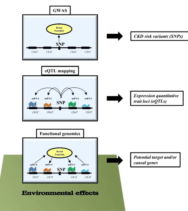
Figure 1. Schematic representation of different experimental designs to understand CKD development.
Genome-wide association studies (GWASs) examine the relationship between genetic variants (SNP, single nucleotide polymorphism) and disease state (CKD, chronic kidney disease). The eQTL (expression quantitative trait loci) analysis examines the relationship between transcript levels and genetic variations. The relationship between transcript levels around CKD risk variants and kidney function can be studied by functional genomics, by examining the contribution of genetic and environmental factors. CRAT: CKD risk associated transcripts
14 3.2.4. Other methods of CKD research
High-throughput omics datasets can be integrated to complex phenotypic disease signatures with the help of “top-down” systems biology approaches and reconstruct protein-protein interactions. Meanwhile, comprehensive molecular data from basic science (“bottom-up”) are also important to understand the development of a disease (47).
In basic science, several methods can help to understand CKD development, from kidney cell cultures to animal models. For example, there are several animal models used to understand diabetic nephropathy (e.g. Streptozotocin-induced diabetic animals, Akita diabetic mice, db/db mice, Zucker diabetic fatty rats, Wistar fatty rats, etc.). The perfect animal model should exhibit progressive albuminuria and a decrease in renal function, as well as the characteristic histological changes that are observed in cases of human diabetic nephropathy. A rodent model that strongly exhibits all these features of human diabetic nephropathy has not yet been developed (48,49). Unilateral ureteral obstruction and folic acid induced nephropathy rodent models are also widely used to investigate interstitial fibrosis, beside several other animal models (50).
Recently a new and interesting field has become important part of CKD research:
the epigenetics. Epigenetics is the heritable information during cell division other than the DNA sequence itself. The epigenome can be reshaped by environmental effects and as an “environmental footprint” contribute to the variation of phenotypes. The DNA in the nucleus has a highly-organized form wrapped around by proteins called histones. The state of its structure can guide transcriptional factor binding. Different stress factors from the environment can affect the epigenome through cytosine methylation (and other modification of cytosine) and histone-tail modifications. The presence of specific histone- tail modifications can identify cell-type specific gene regulatory regions, such as promoters, enhancers, silencers and insulators. As mentioned above, with the ChIP-Seq method these specific histone-tail proteins can be found, providing a map of the potential localization of the gene regulatory regions (44).
While the ENCODE project did not include kidney cell lines, there are studies examining the epigenetics of the kidney in CKD. For example, a genome-wide cytosine methylation analysis of control and diseased kidney epithelial cells was performed by Ko et al., and more than 4000 differentially methylated regions were found in CKD samples,
15
most of them in developmental and fibrosis-related DNA regions. These differentially methylated regions were enriched not on promoter, but on enhancer regions (51).
In summary, understanding the development of chronic kidney disease and the underlying mechanisms are challenging. Chronic kidney disease is a very complex trait;
therefore, CKD research requires complexity itself. The methodology of CKD research needs to include both basic science through cell lines and animal models and high- throughput technologies with genome-, epigenome- and transcriptome-wide studies. In this Ph.D. work, I used functional genomic approaches to prioritize potentially important transcripts in CKD development.
16
4. Objectives
We hypothesized that polymorphisms associated with renal disease will influence the expression of nearby transcript levels in the kidney. In this Ph.D. work, I mapped the expression of these transcripts in normal and disease human kidney samples. I used functional genomics and systems biology approaches to investigate tissue-specific expression of transcripts and their correlation with kidney function.
The goals of the Ph.D. work were:
1. Providing a dataset of potential causal and/or target genes in the vicinity of the CKD risk associated loci
2. Identifying critical pathways associated with kidney function decline for further analysis
17
5. Methods
5.1. Human kidney samples
5.1.1. Tissue handling and microdissection
The human kidney samples were obtained from routine surgical nephrectomies.
For RNA sequencing analysis, leftover portions of diagnostic kidney biopsies were used (n=2). Only the normal, non-neoplastic part of the tissue was used for further investigation. Samples were de-identified, and corresponding clinical information was collected by an individual who was not involved in the research protocol. The tissue and data collecting procedure was approved by the institutional review boards (IRBs) of the Albert Einstein College of Medicine and Montefiore Medical Center, Bronx, NY, USA (IRB 2002–202) and the University of Pennsylvania, Philadelphia, PA, USA (IRB 815796).
The fresh kidney tissue was immediately placed and stored in RNAlater solution (Thermo Fisher Scientific, Ambion, Waltham, MA, USA) according to the manufacturer’s instruction: the tissue was cut into pieces -smaller than 0.5 cm in any dimension- and stored at 4 ℃ overnight, allowing the solution to penetrate the whole tissue. We stored the samples in RNAlater solution at -80 ℃ until the experiments.
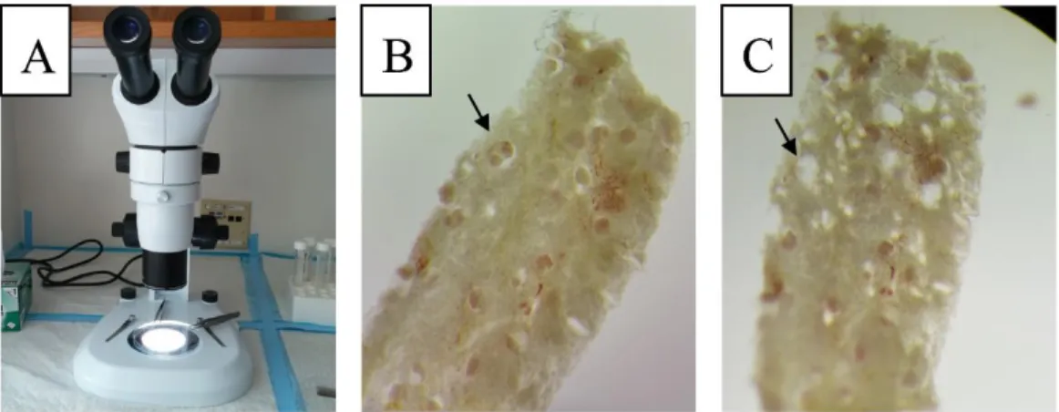
Before the RNA (ribonucleic acid) isolation, the kidney tissue in RNAlater solution was manually microdissected for glomerular and tubular compartment under a microscope. Using fine forceps, the glomeruli were removed from the kidney tissue and processed separately. We refer the rest of the kidney tissue as “tubules”, however, it contains not only tubules but other kind of tissues, e.g. vessels and connective tissue.
(Figure 2.)
5.1.2. Sample characteristics
To examine gene expression changes, we extracted RNA form 95 tubule samples and 51 glomeruli samples, furthermore, 41 tubule samples were used for external validation. The kidney samples were obtained from a diverse population, samples from patients of different age, gender, ethnicity with hypertensive or diabetic nephropathy were examined. Our dataset contains samples from non-Hispanic white,
18
Figure 2. Microdissection of human kidney samples stabilized in RNAlater
Microscope and forceps used for microdissection (A). Intact human kidney sample -glomerulus (arrow) (B). Several glomeruli were removed (arrow) (C)
African American, Asian, Hispanic and multiracial race, so we examined our dataset to exclude any ethnicity driven gene expression changes. We performed statistical analysis (one-way ANOVA – analysis of variance) to identify gene expression differences driven by ancestry in our database. We compared gene expression profiles of kidneys obtained from non-Hispanic white, African American and other ethnicities, and were unable to identify transcripts with statistically significant differential expression in our data.
(Expression profiles of 95 tubule samples and 51 glomerular samples were examined.) (Table 1.). Review of the literature also failed to identify ancestry specific gene expression differences. Therefore, we believe that race is not a critical driver of gene expression differences in our dataset.
The main part of our analysis was examining gene expression correlation with renal function (based on estimated glomerular filtration rate (eGFR) according to the Chronic Kidney Disease Epidemiology Collaboration [CKD-EPI] determination (52)), therefore, we analyzed the correlation between eGFR and clinical and histopathological changes, to exclude any unexpected correlations in our dataset. As expected, we found significant correlation between eGFR and serum creatinine levels, blood urea nitrogen levels (BUN), the percentage of glomerulosclerosis and interstitial fibrosis. On the other hand, we failed to detect any significant correlation between renal function (eGFR) and age, serum glucose levels, serum albumin levels and body mass index (BMI). The demographics, clinical information and histopathological analysis of the samples are summarized in Table 2 (a-d).
19
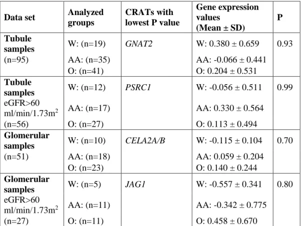
Table 1. Gene expression is not driven by ancestry in our microarray data sets Statistical analysis (one-way ANOVA) between three ethnic groups (non-Hispanic white vs. African American vs. other ethnicity) was performed to search for differentially expressed transcripts. We failed to detect any significant gene expression changes among CRATs (CKD-risk associated transcripts) and among all entities (not shown). eGFR:
glomerular filtration rate, SD: standard deviation, P: P-values after Benjamini- Hochberg-based multiple testing correction, W: non-Hispanic white, AA: African American, O: Other ethnicity, GNAT2: G Protein Subunit Alpha Transducin 2, PSRC1:
Proline and Serine Rich Coiled-Coil 1, CELA2A/B:Chymotrypsin Like Elastase Family Member 2A/B, JAG1: Jagged 1
Data set Analyzed groups
CRATs with lowest P value
Gene expression values
(Mean ± SD)
P Tubule
samples W: (n=19) GNAT2 W: 0.380 ± 0.659 0.93
(n=95) AA: (n=35) AA: -0.066 ± 0.441
O: (n=41) O: 0.204 ± 0.531
Tubule
samples W: (n=12) PSRC1 W: -0.056 ± 0.511 0.99 eGFR>60
ml/min/1.73m2 AA: (n=17) AA: 0.330 ± 0.564
(n=56) O: (n=27) O: 0.113 ± 0.494
Glomerular
samples W: (n=10) CELA2A/B W: -0.115 ± 0.104 0.70
(n=51) AA: (n=18) AA: 0.059 ± 0.204
O: (n=23) O: 0.140 ± 0.244
Glomerular
samples W: (n=5) JAG1 W: -0.557 ± 0.341 0.80 eGFR>60
ml/min/1.73m2 AA: (n=11) AA: -0.342 ± 0.775
(n=27) O: (n=11) O: 0.458 ± 0.670
20
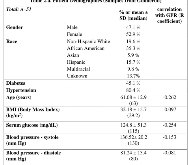
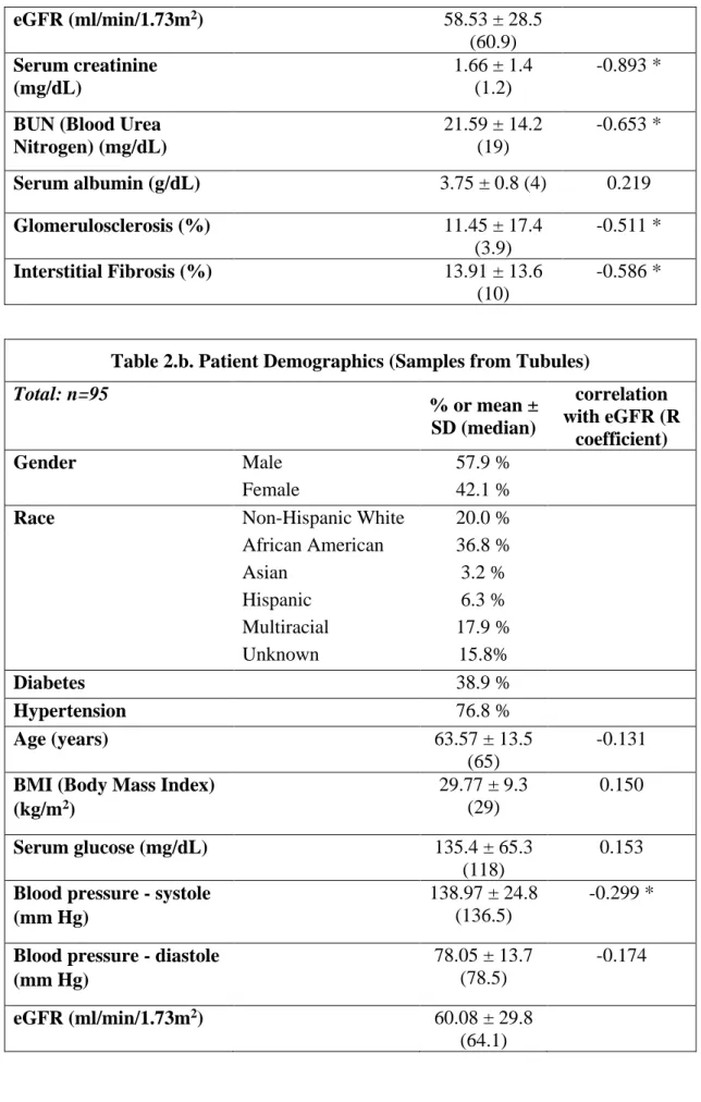
Table 2. Demographics, clinical information and histological analysis of glomerular samples (a), tubule samples (b), tubule samples of the external microarray validation (c), tubule samples of the QRT-PCR validation (d)
Data are presented as mean and standard deviation with the median values or percentage.
Estimated Glomerular Filtration Rate (eGFR) was calculated according to the CKD-EPI equation. Pearson product moment correlation or Spearman correlation coefficient (R coefficient) was used to measure the strength of association between age, BMI (body mass index), serum-glucose, blood pressure (systole and diastole), serum-creatinine, BUN (blood urea nitrogen), serum-albumin, percentage of glomerulosclerosis and interstitial fibrosis and eGFR; depending on the results of the D'Agostino-Pearson normality tests. Asterisks (*) indicate when the two-tailed tests reached statistical significance (P < 0.05).
Table 2.a. Patient Demographics (Samples from Glomeruli) Total: n=51
% or mean ± SD (median)
correlation with GFR (R
coefficient)
Gender Male 47.1 %
Female 52.9 %
Race Non-Hispanic White 19.6 %
African American 35.3 %
Asian 5.9 %
Hispanic 15.7 %
Multiracial 9.8 %
Unknown 13.7%
Diabetes 45.1 %
Hypertension 80.4 %
Age (years)
61.08 ± 12.9 (63)
-0.262 BMI (Body Mass Index)
(kg/m2)
32.18 ± 15.7 (29.2)
-0.097
Serum glucose (mg/dL)
124.8 ± 51.3 (115)
-0.254 Blood pressure - systole
(mm Hg)
136.52± 20.2 (130)
-0.153
Blood pressure - diastole (mm Hg)
81.24 ± 13.4 (80)
-0.081
21 eGFR (ml/min/1.73m2)
58.53 ± 28.5 (60.9) Serum creatinine
(mg/dL)
1.66 ± 1.4 (1.2)
-0.893 *
BUN (Blood Urea Nitrogen) (mg/dL)
21.59 ± 14.2 (19)
-0.653 *
Serum albumin (g/dL)
3.75 ± 0.8 (4) 0.219 Glomerulosclerosis (%)
11.45 ± 17.4 (3.9)
-0.511 * Interstitial Fibrosis (%)
13.91 ± 13.6 (10)
-0.586 *
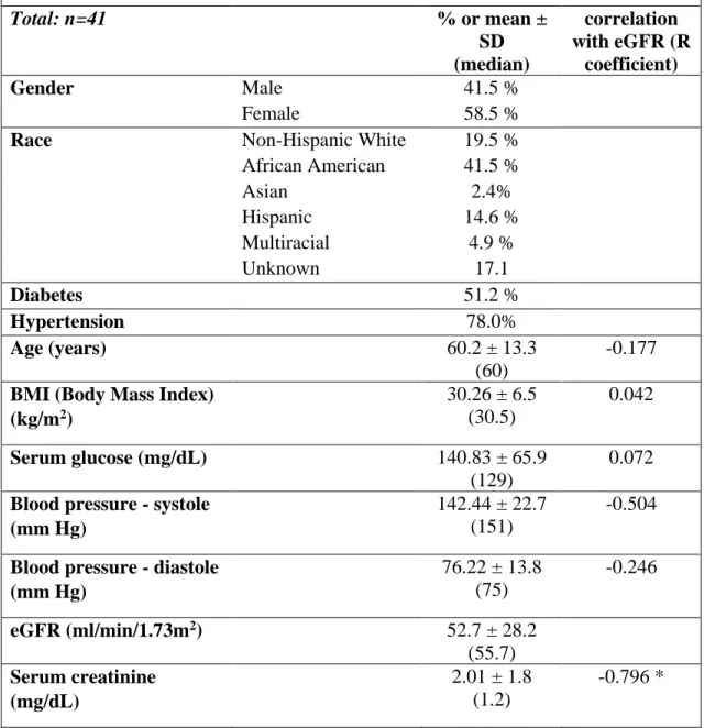
Table 2.b. Patient Demographics (Samples from Tubules) Total: n=95
% or mean ± SD (median)
correlation with eGFR (R
coefficient)
Gender Male 57.9 %
Female 42.1 %
Race Non-Hispanic White 20.0 %
African American 36.8 %
Asian 3.2 %
Hispanic 6.3 %
Multiracial 17.9 %
Unknown 15.8%
Diabetes 38.9 %
Hypertension 76.8 %
Age (years) 63.57 ± 13.5
(65)
-0.131 BMI (Body Mass Index)
(kg/m2)
29.77 ± 9.3
(29)
0.150
Serum glucose (mg/dL) 135.4 ± 65.3 (118)
0.153 Blood pressure - systole
(mm Hg)
138.97 ± 24.8
(136.5)
-0.299 *
Blood pressure - diastole (mm Hg)
78.05 ± 13.7
(78.5)
-0.174
eGFR (ml/min/1.73m2) 60.08 ± 29.8 (64.1)
22 Serum creatinine
(mg/dL)
2.05 ± 2.5
(1.1)
-0.894 *
BUN (Blood Urea Nitrogen) (mg/dL)
23.2 ± 13.7
(19)
-0.696 *
Serum albumin (g/dL) 3.96 ± 0.7
(4.1)
0.228 * Glomerulosclerosis (%) 17.97 ± 27.3
(5.5)
-0.570 * Interstitial Fibrosis (%) 16.47 ± 21.6
(10)
-0.732 *
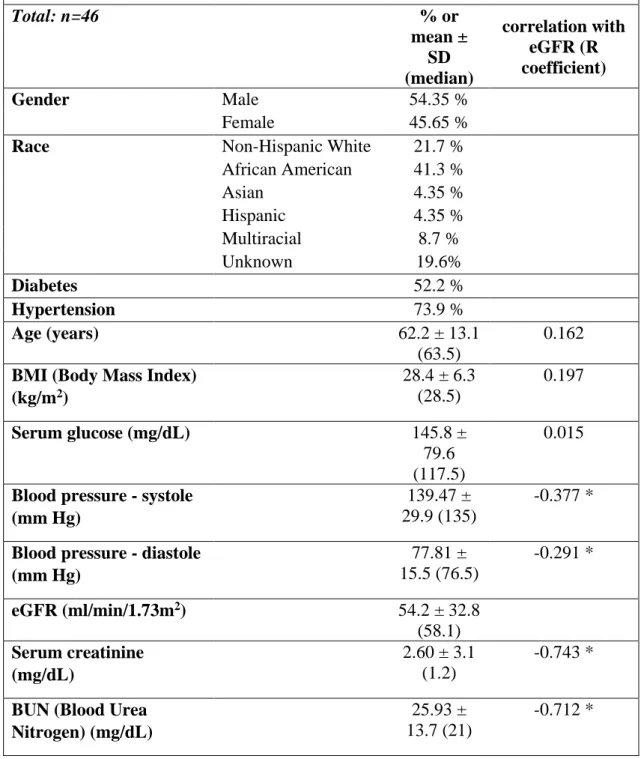
Table 2.c. Patient Demographics (Samples from Tubules for Replication)
Total: n=41 % or mean ±
SD (median)
correlation with eGFR (R
coefficient)
Gender Male 41.5 %
Female 58.5 %
Race Non-Hispanic White 19.5 %
African American 41.5 %
Asian 2.4%
Hispanic 14.6 %
Multiracial 4.9 %
Unknown 17.1
Diabetes 51.2 %
Hypertension 78.0%
Age (years) 60.2 ± 13.3
(60)
-0.177 BMI (Body Mass Index)
(kg/m2)
30.26 ± 6.5
(30.5)
0.042
Serum glucose (mg/dL) 140.83 ± 65.9 (129)
0.072 Blood pressure - systole
(mm Hg)
142.44 ± 22.7
(151)
-0.504
Blood pressure - diastole (mm Hg)
76.22 ± 13.8
(75)
-0.246
eGFR (ml/min/1.73m2) 52.7 ± 28.2 (55.7) Serum creatinine
(mg/dL)
2.01 ± 1.8
(1.2)
-0.796 *
23 BUN (Blood Urea
Nitrogen) (mg/dL)
25.0 ± 13.1
(22)
-0.749 *
Serum albumin (g/dL) 3.69 ± 0.9
(3.9)
0.409 * Glomerulosclerosis (%) 17.97 ± 25.5
(14.3)
-0.641 * Interstitial Fibrosis (%) 19.93 ± 22.0
(15)
-0.769 *
Table 2.d. Patient Demographics (Tubule samples with QRT-PCR validation)
Total: n=46 % or
mean ± SD (median)
correlation with eGFR (R coefficient)
Gender Male 54.35 %
Female 45.65 %
Race Non-Hispanic White 21.7 %
African American 41.3 %
Asian 4.35 %
Hispanic 4.35 %
Multiracial 8.7 %
Unknown 19.6%
Diabetes 52.2 %
Hypertension 73.9 %
Age (years) 62.2 ± 13.1
(63.5)
0.162 BMI (Body Mass Index)
(kg/m2)
28.4 ± 6.3
(28.5)
0.197
Serum glucose (mg/dL) 145.8 ±
79.6 (117.5)
0.015
Blood pressure - systole (mm Hg)
139.47 ±
29.9 (135)
-0.377 *
Blood pressure - diastole (mm Hg)
77.81 ±
15.5 (76.5)
-0.291 *
eGFR (ml/min/1.73m2) 54.2 ± 32.8 (58.1) Serum creatinine
(mg/dL)
2.60 ± 3.1
(1.2)
-0.743 *
BUN (Blood Urea Nitrogen) (mg/dL)
25.93 ±
13.7 (21)
-0.712 *
24
Serum albumin (g/dL) 3.94 ± 0.6
(4)
0.064 Glomerulosclerosis (%) 23.7 ± 33.1
(6.2)
-0.748 * Interstitial Fibrosis (%) 21.53 ±
25.3 (10)
-0.737 *
5.2. Sample processing and data analysis 5.2.1. Microarray process and data analysis
Dissected tissue was homogenized, and RNA was prepared using RNAeasy mini columns (Qiagen, Valencia, CA, USA) according to the manufacturer’s instructions: the tissue was placed in the lysis buffer and homogenized with an Omni Tissue Homogenizer (Omni, Kennesaw, GA, USA). DNase (deoxyribonuclease) digestion was used as an additional step to improve RNA purification. RNA quality and quantity were determined using the Laboratory-on-Chip Total RNA PicoKit Agilent 2100 BioAnalyzer (Agilent Technologies, Santa Clara, CA, USA). Only samples without evidence of degradation were further used (RNA integrity number [RIN] >6).
For microarray analysis, we prepared the first and second strand of the complementary DNA (cDNA) and after amplification, purification and cDNA fragmentation, we labelled the cDNA fragments. Purified total RNAs from 95 tubule samples were amplified using the Ovation PicoWTA SystemV2 (NuGEN Technologies, San Carlos, CA, USA) and labeled with the Encore Biotin Module (NuGEN) according to the manufacturer’s protocol. The purified total RNAs from 51 glomerular samples and 41 tubule samples used for validation were amplified using the Two-Cycle Target LabelingKit (Affymetrix, Santa Clara, CA, USA) as per the manufacturer’s protocol.
Transcript levels were analyzed using Affymetrix U133A arrays.
After hybridization and scanning on microarray chips, raw data files were imported into GeneSpring GX software, version 12.6 (Agilent Technologies). Raw expression levels were summarized using the RMA16 (Robust Multi-Array Average) algorithm. Normalized values were generated after log transformation and baseline transformation. GeneSpring GX software then was used for statistical analysis.
25 5.2.2. RNA sequencing analysis
RNA sequencing was carried out on microdissected kidney tubules from kidney biopsies. Total RNA was isolated using the RNeasy mini columns (Qiagen) according to the manufacturer’s protocol, as described above. An additional DNase digestion step was performed to ensure that the samples were not contaminated with genomic DNA. RNA purity was assessed using the Laboratory-on-Chip Total RNA PicoKit Agilent 2100 BioAnalyzer (Agilent Technologies). Each RNA sample had an A260:A280 ratio 1.8 and an A260:A230 ratio 2.2, with an RIN>9.0. Single-end 100-basepair RNA sequencing was carried out an Illumina HiSeq2000 machine (Illumina, San Diego, CA, USA). RNA sequencing reads were aligned to the human genome (GRCh37/hg19, University of California Santa Cruz [UCSC]) with the software TopHat (version 2.0.9) and transcriptome (hg19 RefSeq from Illumina iGenomes) using the software Cufflinks (version 2.1.1 Linux_x86_64) (53,54). We counted the number of fragments mapped to each gene annotated in the UCSC hg19. Transcript abundances were measured in Fragments Per Kilobase of transcript per Million mapped reads (FPKM). Sequence data can be accessed at the National Center for Biotechnology Information’s Gene Expression Omnibus (Accession number: GSE60119).
5.2.3. Quantitative real time polymerase chain reaction (QRT-PCR) analysis
Using reverse transcriptase, 250 ng RNA was converted to cDNA using the cDNA Archive Kit (Thermo Fisher Scientific, Applied Biosystems, Waltham, MA, US) and QRT-PCR was run in the ViiA 7 System (Applied Biosystems) machine using SYBR Green Master Mix (Applied Biosystems) and gene-specific primers. The data were normalized and analyzed using the ΔΔCT method, ubiquitin was used as a housekeeping gene for normalization.
5.2.4. Genotyping of human kidney samples
After the disruption and homogenization of the human kidney tissue as described above, DNA was extracted and purified with the DNeasy Blood and Tissue Kit (Qiagen), according to the manufacturer’s protocol. Genotyping for rs881858 and rs6420094 loci was run in the ViiA 7 System (Applied Biosystems) machine using TaqMan Genotyping Master Mix (Applied Biosystems) and specific TaqMan assay probes.
26 5.2.5. Histology
Glomerular sclerosis and interstitial fibrosis were evaluated using periodic acid–
Schiff-stained kidney sections by two independent nephropathologists.
Immunohistochemistry was performed on paraffin-embedded sections with the following antibodies: UMOD (AAH35975, Sigma Aldrich, St. Louis, MO, USA), VEGFA (Ab46154, Abcam, Cambridge, MA, USA) and ACSM2A (Ab181865, Abcam).
We used the Vectastain Mouse on Mouse or anti-rabbit Elite ABC Peroxidase Kit and 3,3’diaminobenzidine (DAB) for visualizations (Vector Laboratories, Burlingame, CA, USA). Antibody specificity was evaluated separately; secondary antibodies alone showed no positive staining.
5.3. Bioinformatics
5.3.1. Gene ontology and network analyses
We performed gene ontology analysis on the CKD risk associated transcripts of interest, using the Database for Annotation, Visualization and Integrated Discovery (DAVID) Bioinformatics Resources, available on-line at david.abcc.ncifcrf.gov. (55,56)
To perform network analysis on the transcripts with expression levels showing significant linear correlation with eGFR, the transcripts were exported to the Ingenuity Pathway Analysis (IPA) software (Ingenuity Systems, Qiagen). This software determines the top canonical pathways by using a ratio (calculated by dividing the number of genes in each pathway that meet cutoff criteria by the total number of genes that constitute that pathway) and then scoring the pathways using a Fisher exact test (P value < 0.05).
5.3.2. Processing publicly available datasets
We compared absolute expression levels of the transcripts of interest by processing the data of the publicly available Illumina Body Map database (The European Bioinformatics Institute, www.ebi.ac.uk) which provides RNA sequencing results in 16 different human organs.
For additional expression quantitative trait loci (eQTL) analysis, we examined multiple different datasets with the help of the publicly available eQTL browser at www.ncbi.nlm.nih.gov. These datasets included the MuTHER (Multiple Tissue Human
27
Expression Resource) and other studies, where transcript levels were available from liver, adipose, and lymphoblastoid samples (42,57-60).
For evaluation of the expressions of the genes of interest on protein level, additional to our own immunohistochemistry results, we reviewed the publicly available data of The Human Protein Atlas (www.proteinatlas.org) (61).
5.4. Overview of the used statistical methods
For statistical analysis of the demographic, clinical and histopathological parameters, Pearson product moment correlation or Spearman correlation coefficient (R coefficient) was used to measure the strength of association between age, BMI (body mass index), serum-glucose, blood pressure (systole and diastole), serum-creatinine, BUN (Blood urea nitrogen), serum-albumin, percentage of glomerulosclerosis and interstitial fibrosis and eGFR; depending on the results of the D'Agostino-Pearson normality tests. The statistical significance of the correlation was calculated with two- tailed test (alpha=0.05). To compare the expression of the genotyped samples in our eQTL analysis, one-way ANOVA and Student’s t-test were used. The statistical analyses were performed using Prism 6 software (GraphPad, La Jolla, CA, USA).
GeneSpring GX software was used for statistical analysis to process microarray data. Pearson product moment correlation was used to measure the strength of association between gene expression and eGFR. We used Benjamini–Hochberg multiple testing correction with a P value of 0.05. In the case of genes with more probe set identifications, the results with the lowest P values are represented.
28
6. Results
6.1. Identifying CKD risk associated transcripts (CRATs)
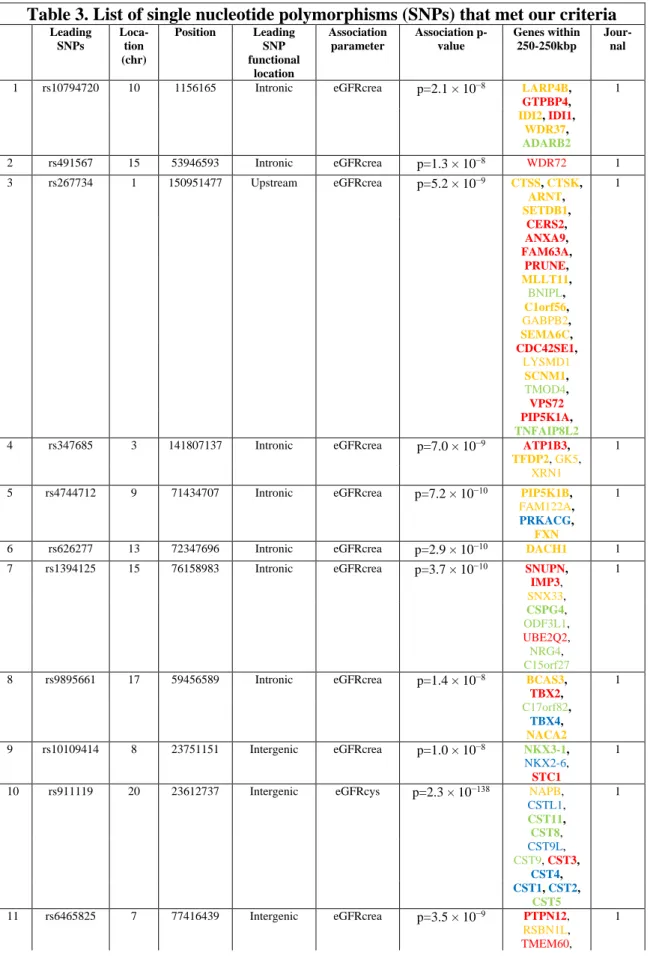
To identify CKD risk associated transcripts, we performed manual literature search to examine all genome-wide association studies - by the time of the beginning of our study- reporting genetic association for CKD-related traits (9-28,30-33). Many of these studies used different parameters as kidney disease indicators, such as the serum creatinine or cystatin C levels, the presence of CKD or end stage renal disease (ESRD) or albuminuria/proteinuria. In our investigation, the SNPs associated with eGFR (based on serum creatinine or cystatin C calculations) or the presence of ESRD were included. Our literature analysis identified 10 publications meeting these criteria (9-15,18-20). Coding polymorphisms and SNPs that did not reach genome-wide significance (P > 5 x 10⁻⁸) were excluded from our study. Finally, 44 leading SNPs meeting these criteria were used for further analysis (Table 3.). Most publications did not differentiate cases based on disease etiology and included cases with hypertensive and diabetic kidney disease, nevertheless, three SNPs associated only with diabetic nephropathy, so they were also analyzed separately. There were only two SNPs that reached genome-wide significance in multiple studies (rs12917707 and rs9895661), these two SNPs were counted only once.
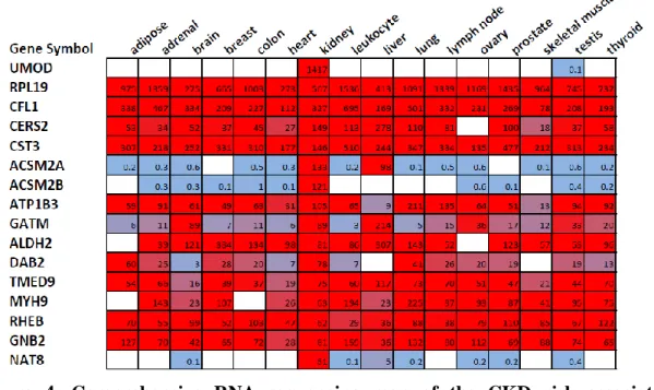
Table 3. List of single nucleotide polymorphisms (SNPs) that met our criteria The table shows the list of the single nucleotide polymorphisms (SNPs) which reached the genome wide significance (P < 5 x 10⁻⁸) in the association with eGFR (estimated glomerular filtration rate, based on creatinine (crea) or cystatin C (cys) levels) and/or the presence of chronic kidney disease (CKD) or end stage renal disease (ESRD). SNPs which reached the genome-wide significance in multiple studies were counted only once (marked with “X” in the table). Genes less than 250 kbp (kilobase pair) from the leading SNPs are listed. Color-coding shows the baseline expression of the transcripts based on human kidney RNA sequencing, red: high expression, yellow: medium expression, green:
low expression, blue: no expression. Genes with available probe set IDs on the microarray chip are marked bold. Gene symbols are official symbols approved by the Human Genome Organization Gene Nomenclature Committee (HGNC). Chr: chromosome
29
Table 3. List of single nucleotide polymorphisms (SNPs) that met our criteria
Leading SNPs
Loca- tion (chr)
Position Leading
SNP functional
location
Association parameter
Association p- value
Genes within 250-250kbp
Jour- nal
1 rs10794720 10 1156165 Intronic eGFRcrea p=2.1 × 10⁻⁸ LARP4B,
GTPBP4, 1
IDI2, IDI1, WDR37,
ADARB2
2 rs491567 15 53946593 Intronic eGFRcrea p=1.3 × 10⁻⁸ WDR72 1
3 rs267734 1 150951477 Upstream eGFRcrea p=5.2 × 10⁻⁹ CTSS, CTSK,
ARNT, SETDB1,
1
CERS2,
ANXA9, FAM63A,
PRUNE,
MLLT11, BNIPL,
C1orf56,
GABPB2, SEMA6C,
CDC42SE1,
LYSMD1
SCNM1,
TMOD4, VPS72 PIP5K1A, TNFAIP8L2
4 rs347685 3 141807137 Intronic eGFRcrea p=7.0 × 10⁻⁹ ATP1B3,
TFDP2, GK5, 1
XRN1
5 rs4744712 9 71434707 Intronic eGFRcrea p=7.2 × 10⁻¹⁰ PIP5K1B,
FAM122A, 1
PRKACG,
FXN
6 rs626277 13 72347696 Intronic eGFRcrea p=2.9 × 10⁻¹⁰ DACH1 1
7 rs1394125 15 76158983 Intronic eGFRcrea p=3.7 × 10⁻¹⁰ SNUPN,
IMP3, SNX33,
1
CSPG4, ODF3L1, UBE2Q2, NRG4, C15orf27
8 rs9895661 17 59456589 Intronic eGFRcrea p=1.4 × 10⁻⁸ BCAS3,
TBX2,
1
C17orf82,
TBX4, NACA2
9 rs10109414 8 23751151 Intergenic eGFRcrea p=1.0 × 10−8 NKX3-1,
NKX2-6, STC1
1
10 rs911119 20 23612737 Intergenic eGFRcys p=2.3 × 10−138 NAPB,
CSTL1, CST11, CST8,
1
CST9L,
CST9, CST3, CST4,
CST1, CST2,
CST5
11 rs6465825 7 77416439 Intergenic eGFRcrea p=3.5 × 10⁻⁹ PTPN12,
RSBN1L, TMEM60,
1
30
PHTF2,
MAGI2
12 rs653178 12 112007756 Intronic eGFRcys p=3.8 × 10−8 CUX2,
FAM109A, SH2B3,
1
ATXN2,
BRAP, ACAD10,
ALDH2
13 rs6420094 5 176817636 Intronic eGFRcrea p=3.8 × 10⁻¹² NSD1,
RAB24, PRELID1,
1
MXD3,
LMAN2, RGS14,
SLC34A1,
PFN3,
F12, GRK6,
PRR7,
DBN1,
PDLIM7, DOK3,
DDX41,
FAM193B, TMED9,
B4GALT7
14 rs11959928 5 39397132 Intronic eGFRcrea p=1.8 × 10⁻¹¹ FYB, C9,
DAB2
1
15 rs12917707 16 20367690 Upstream eGFRcrea p=1.2 × 10⁻²⁰ GP2, UMOD,
PDILT, ACSM5, ACSM2A,
ACSM2B 1
16 rs2453533 15 45641225 Intergenic eGFRcrea p=4.6 × 10−22 DUOX1,
DUOXA2, DUOXA1,
1
SHF,
SLC28A2, GATM,
SPATA5L1,
C15orf48,
SLC30A4,
BLOC1S6
17 rs17319721 4 77368847 Intronic eGFRcrea p=1.1 × 10⁻¹⁹ SCARB2,
FAM47E, 1
STBD1,
CCDC158,
SHROOM3
18 rs1933182 1 109999588 Intergenic eGFRcrea p=1.3 × 10⁻⁸ SARS,
CELSR2, PSRC1,
1
MYBPHL,
SORT1, PSMA5,
SYPL2,
ATXN7L2, CYB561D1,
AMIGO1,
GPR61, GNAI3,
AMPD2,
GSTM2, GSTM4,
GSTM1,
GNAT2
19 rs16864170 2 5907880 Intergenic CKD p=4.5 × 10−8 SOX11 1
20 rs881858 6 43806609 Intergenic eGFRcrea p=2.2 × 10⁻¹¹ POLH,
GTPBP2, MAD2L1BP,
1
31
RSPH9,
MRPS18A, VEGFA,
C6orf223
21 rs7805747 7 151407801 Intronic CKD p=8.6 × 10⁻⁹ RHEB,
PRKAG2 1
22 rs4014195 11 65506822 Intergenic eGFRcrea p=3.3 × 10⁻⁸ SCYL1,
LTBP3, SSSCA1,
1
FAM89B,
EHBP1L1, KCNK7,
MAP3K11,
PCNXL3, SIPA1,
RELA,
KAT5, RNASEH2C,
AP5B1,
OVOL1, SNX32,
CFL1,
MUS81, EFEMP2,
CCDC85B,
FOSL1, CTSW,
FIBP,
C11orf68, TSGA10IP,
SART1,
DRAP1
23 rs12460876 19 33356891 Intronic eGFRcrea p=5.5 × 10⁻⁹ ANKRD27,
RGS9BP, 1
NUDT19,
TDRD12, SLC7A9,
CEP89,
C19orf40, RHPN2,
GPATCH1
24 rs2279463 6 160668389 Intronic eGFRcrea p=8.7 × 10⁻¹⁰ IGF2R,
SLC22A1, SLC22A2,
1
SLC22A3
25 rs10774021 12 349298 Intronic eGFRcrea p=6.7 × 10⁻⁹ IQSEC3,
SLC6A12, SLC6A13,
1
KDM5A,
CCDC77,
B4GALNT3
26 rs6431731 2 15863002 Intergenic eGFRcrea p=4.6 x 10-8 DDX1,
MYCN
2
27 rs3925584 11 30760335 Intergenic eGFRcrea p=1 x 10⁻⁹ MPPED2,
DCDC5, DCDC1
2
28 rs12124078 1 15869899 Intronic eGFRcrea p=9.8 x 10⁻¹⁰ FHAD1,
EFHD2, CTRC,
2
CELA2A,
CELA2B, CASP9,
DNAJC16,
AGMAT, DDI2,
RSC1A1,
SLC25A34,
TMEM82,
FBLIM1
32
29 rs2453580 17 19438321 Intronic eGFRcrea p=4.6 x 10⁻⁸ EPN2, B9D1,
MAPK7,
2
MFAP4,
RNF112, SLC47A1,
ALDH3A2,
ALDH3A1,
SLC47A2,
ULK2
30 rs11078903 17 37631924 Intronic eGFRcrea p=2.4 x10⁻⁹ FBXL20,
MED1, CDK12,
2
NEUROD2,
PPP1R1B,
STARD3,
PNMT, PGAP3,
ERBB2,
TCAP
31 rs4293393 16 20364588 Intronic eGFRcrea p=2.6 x10⁻¹⁰ GP2, UMOD,
PDILT,
3
ACSM5,
ACSM2A, ACSM2B
X rs12917707 16 20367690 Intronic CKD p=2.9 x 10⁻⁹ GP2, UMOD,
PDILT,
4
ACSM5,
ACSM2A, ACSM2B
32 rs6040055 20 10633313 Intronic eGFRcrea p=1 x 10⁻⁸ MKKS,
SLX4IP, JAG1
4
33 rs1731274 8 23766319 Intergenic eGFRcys p=4.6 x 10⁻⁸ STC1, NKX3-
1, NKX2-6 4
34 rs13038305 20 23610262 Intronic eGFRcys p=2.2 x 10-88 NAPB,
CSTL1, CST11, CST8,
4
CST9L,
CST9, CST3, CST4,
CST1, CST2,
CST5
35 rs10206899 2 73900900 Intronic eGFRcrea p=2.3 x 10⁻⁸ ALMS1,
NAT8, NAT8B,
5
TPRKB,
DUSP11, C2orf78,
STAMBP,
ACTG2
X rs9895661 17 59456589 Intronic eGFRcrea p=4.8 × 10⁻¹¹ BCAS3,
TBX2,
6
C17orf82,
TBX4, NACA2
36 rs11864909 16 20400839 Intronic eGFRcrea p=3.6 × 10⁻¹⁰ GP2, UMOD,
PDILT,
6
ACSM5,
ACSM2A, ACSM2B,
ACSM1
37 rs13146355 4 77412140 Intronic eGFRcrea p=6.6 × 10⁻¹¹ FAM47E,
STBD1,
6
CCDC158,
SHROOM3
38 rs10277115 7 1285195 Intergenic eGFRcrea p=1.0 × 10⁻¹⁰ C7orf50,
GPR146, GPER,
6