Hybrid time-quality-cost trade-off problems

Hybrid time-quality-cost trade-off problems

Zsolt T. Koszty´an¹, Istv´an Szalkai²

1Department of Quantitative Methods,²Department of Mathematics,

1−2University of Pannonia, Hungary

Abstract

Agile and hybrid project management has become increasingly popular among practitioners, particularly in the IT sector. In contrast to the theoreti- cally and algorithmically well-established and developed time-cost and time- quality-cost project management methods, agile and hybrid project manage- ment lacks a principle foundation and algorithmic treatment. The aim of this paper is to fill this gap. We propose a matrix-based method that provides scores for alternative project plans that host flexible task dependencies and undecided, supplementary task completion while also covering traditional time-quality-cost trade-off problems. The proposed method can bridge the agile and traditional approaches.

Keywords: Time-quality-cost trade-off problems, Hybrid project management approaches, Matrix-based project planning

1. Introduction

The importance of time-cost trade-off problems was recognized over five decades ago, with the nearly simultaneous development of project planning techniques [1]. From the 1960s to the 1980s, continuous time-cost relation- ship problems were addressed extensively in the literature [see, e.g., 2, 3].

The discrete time-cost trade-off problem (DTCTP), which can be treated as a specific resource-allocation problem [4], is a well-known problem in the project management literature [see, e.g., 5, 6, 7]. At first, Ref. [8] suggested that the quality of a completed project may be affected by project crash- ing. They developed a solution procedure that considers trade-offs among time, cost and quality in a continuous mode. Since discrete time-cost trade- off problems (DTCTP) are NP-hard problems, discrete time-quality-cost trade-off problems (DTQCTP) are also NP-hard problems and are therefore

usually solved using heuristic or meta-heuristic methods. However, contin- uous versions of these problems can usually be solved within a polynomial computational time (e.g., in the case of linear trade-off functions between time-cost and time-quality) [9]. All of these problems assume a fixed-logic plan, whereas recent project management (e.g., agile and hybrid) approaches allow for the restructuring or reorganization of the project. They approaches apply flexible-logic plans instead of fixed-logic plans. This paper extends the traditional trade-off problem to address flexible project plans.

Continuous and discrete versions of time-cost and time-quality-cost trade- off analyses assume that the time, cost and quality of an option within an activity are deterministic. However, the time, quality and cost may be un- certain. The stochastic versions of time-cost and time-quality-cost trade-off problems [see, e.g., 10, 11] treat time, quality and cost as uncertain param- eters. In the proposed method, the task (e.g., time/cost/resource) demands are not uncertain, but the logical structure is. The proposed model can address uncertainty regarding supplementary task completion and/or un- certain or flexible dependencies.

It is interesting to combine uncertain task durations, uncertain cost de- mands, uncertain quality parameters (undecided), supplementary task com- pletion and uncertain or flexible task dependencies into one stochastic model;

however, this paper mainly focuses on how to extend continuous and dis- crete time-quality-cost trade-off methods to treat flexible dependencies and (undecided or uncertain) supplementary task completion.

Every traditional trade-off method assumes an accepted logic plan by which the tasks and the dependencies between them are determined. How- ever, several project management approaches, e.g., agile and extreme project management (see Ref. [12]), allow for one to restructure or reorganize the project plan in response to changes in the client’s demands.

Wysocki found in a 2009 study of the practices of software project man- agers that only 20% of IT projects were managed using a traditional project management (TPM) methodology. Methods for investment and construc- tion projects usually cannot be directly applied to software development or R&D projects, as these are managed using agile project management (APM) approaches. Currently, hybrid (i.e., combinations of traditional and agile) approaches are becoming increasingly popular [see, e.g., 13, 14]. However, these approaches lack a principled foundation and algorithmic treatment.

The aim of this paper is to fill this gap.

Whereas a project manager who follows a TPM approach uses TCTP/TQCTP method(s) to reduce task duration, an agile project manager tries to restruc- ture the project. The project duration can be reduced without increasing

the project cost by reducing the number of flexible dependencies. However, in real project situations, most dependencies are fixed; therefore, the TPM and APM approaches should be integrated.

There are different combinations of agile and traditional project man- agement approaches [see, e.g., 15, 16, 13]. However, to the best of our knowledge, there is no exact algorithm that can be used to in hybrid time- quality-cost trade-off problems. Nevertheless, production development and IT projects, such as introducing and setting up new information systems, may require that part of the project be reorganized, particularly in the devel- opment phase. However, decreasing the time demands of mandatory tasks may also be an important requirement. Neither the agile nor the traditional approach can address this situation properly. Traditional approaches, or network-based methods, assume static logic plans, but the reorganization of projects may produce insufficient reductions in project duration and/or sup- plementary tasks, and important tasks may be excluded from the project due to budget constraints and/or project deadlines. A hybrid project manage- ment (HPM) approach may combine the traditional and agile approaches;

however, HPM approaches are not yet supported by project planning meth- ods. The proposed algorithm combines the agile and traditional approaches.

This method extends traditional time-cost and time-quality trade-off meth- ods by allowing for the restructuring and reorganizing of projects.

The proposed hybrid time-cost and hybrid time-quality-cost trade-off models manage flexible project plans and allow us to restructure or reorga- nize these project plans to satisfy customer and management demands. In contrast to the traditional project scoring and selection methods, there is no need to specify all project alternatives to select the most desirable project scenario or the one with the shortest duration or lowest cost.

To handle flexible project plans, matrix-based techniques will be used instead of traditional network-based project planning techniques.

The basis of the proposed methods is a matrix-based method, the project domain matrix (PDM) [see 17]. The PDM is an nby mmatrix, wheren is the number of tasks,m=n+t+c+q+r,tis the number of possible durations, cis the number of possible (direct) costs, qis the number of possible quality parameters, andr is the number of possible resource demands of tasks.

The PDM has five domains. The first domain is the logic domain (LD), which is described as an n by n project expert matrix (PEM) [see 18] or numerical dependency structure matrix (NDSM)[see 19]¹. Since the PEM

1The NDSM does not represent supplementary tasks but can represent flexible depen-

has specified and semi-specified versions, the PDM isspecified if and only if the LD is specified; otherwise, the PDM issemi-specified.

The other domains are the time domain (TD), cost domain (CD), qual- ity domain (QD) and resource domain (RD). If the demands are deter- ministic, we say that the PDM is deterministic; otherwise, the PDM is non-deterministic. In this study, the deterministic versions of hybrid time- quality-cost trade-off problems are considered: the TD, CD, QD, and RD contain deterministic values but at least two completion modes. Therefore, this version is a semi-specified, deterministic, multi-modal PDM.

Whereas the basis of the proposed model is the PDM, the basis of the proposed method is the expert project ranking (EPR) algorithm [see 17], which can evaluate specified and semi-specified deterministic PDMs. How- ever, that method cannot address the trade-off problem. Therefore, although EPR can be used to schedule a flexible project plan and can thus be used in agile project management approaches, it cannot address trade-offs between time and cost or between time and quality and therefore cannot be used in hybrid project management directly.

This paper proposes a hybrid time-quality-cost trade-off model to bridge APM and TPM.

The proposed hybrid algorithm combines the features of EPR and time- quality-cost trade-off problems to solve hybrid time-quality-cost trade-off problems.

The proposed algorithm can be used not only for project planning but also for project risk management. Despite risk management and mitigation not being the main focus of this paper, in the section of the simulation beyond traditional risk management, in which project networks are usually assumed to have a fixed logic plan [20] or be a result of a negotiation [21], it was possible to measure the effect of the ratio of flexible dependencies and the ratio of uncertain (supplementary) task completions. The use of flexible dependencies and supplementary tasks enables us to model and compare different project management approaches.

The paper organized as follows: after this section, in Section 2, the mathematical background is described. In Section 3, we present the pro- posed algorithm, and different types of project management approaches are modeled and compared. In the last section (Section 4), we summarize the conclusions and discuss the limitations of the proposed algorithm and future

dencies; however, the PEM can represent both flexible dependencies and supplementary tasks

directions.

2. Solving hybrid time-quality-cost trade-off problems

In this section, a (resource-constrained) hybrid time-quality-cost trade- off problem (RC-HTQCTP) is first specified. Then, a matrix-based model representation is proposed. At the end of this section, an exact algorithm for a hybrid continuous time-quality-cost trade-off problem is proposed. The decisions for finding the optimum will be directed by score functions and matrices (P, Q) and time-quality-cost functions; thus, we need several defi- nitions and notations before proceeding.

2.1. Definitions and problem statements

In the proposed model, mandatory and supplementary activities are dis- tinguished.

Definition 1. We call any finite set A = {a₁, ..., a_n} the set of possible activities or tasks in the project. The subset of supplementary task is Ae={ea₁, ...,ea_σ} ⊆A, where Aeis any fixed subset of A. Then, A=A\Aeis the subset of mandatory tasks.

Whereas mandatory (or high-priority) tasks must be realized, supple- mentary (or lower-priority) tasks can be omitted from the project or post- poned to the next or another project. Decisions aboutsupplementary task realization always have two options: to include or to exclude.

S denotes the set of tasks that will be fulfilled by the algorithm (further- more called as project scenario). The number of possible project scenarios is 2^σ, whereσ =

Ae

.

Definition 2. Any function P :A→[0,1]is called thescore function of task inclusion if P(a_i) = 1 for a_i ∈A and P(a_i)∈[0,1)for a_i ∈A.e The functionQ:A→[0,1]is called thescore function of taskexclusion if Q(ai) = 0 for ai ∈A andQ(ai)∈(0,1] for ai∈A.e

The task inclusion and exclusion scores can mean probability, importance or relative priority values.

Example 1. If every task completion (inclusion) score is a probability value, thenQ= 1−P.

Definition 3. For any associative and monotone² operation ⊗ on R⁺, we define the aggregation function ⊗: Ξ (A)→R as

⊗(S) :=O

a∈S

P(a) ⊗ O

a∈A\S

Q(a), (1)

where⊗ indicates Σ or Π (addition or multiplication, respectively) or ∨or

∧(maximum or minimum, respectively).

Example 2. If scores are probability values, then we have ⊗= Π.

If scores indicate the importance of task completion, then ⊗= Σ.

The phase one of the proposed algorithm decides which tasks will be included in the project scenario by maximizing⊗(S), fulfilling certaintime, quality andcost requirements. Nevertheless, the proposed model also treats flexible relations between two tasks. Therefore, in phase two of the pro- posed algorithm, we decidethe order in which we will complete these tasks.

This order is arelation of tasks, and our algorithm receives three types of re- lations (dependencies) as inputs: no dependency,requiredand flexible.

We have to resolve (i.e., decide) all flexible relations.

Definition 4. The relation triplet(≺,∼,on)is a relation representation of a hybrid project plan if for any i, j≤n and i6=j, we let

(i) ai ≺aj represent the strict or required dependencies between tasks ai

andaj, i.e., aj may not be started unless activity ai has been completed;

(ii) a_i ∼ a_j represents no dependency between tasks a_i and a_j, i.e., the starting time of aj is not affected byai;

(iii)ai onaj represents flexible dependencies between tasks ai and aj. Remark 1. It is important to note that≺is naturally a transitive and asym- metric relation, which excludes circles such as a1 ≺a2 ≺ ...≺ a1. There- fore, by a standard topological ordering algorithm, we may assume that a_i ≺a_j ⇒i < j.

Whereas strict dependency a_i ≺ a_j between tasks a_i and a_j must be realized (in a sequential manner) and ai ∼ aj means indifference (we may choose either sequential or parallel realization), flexible dependencies (on) must be resolved. In this case, we can decide whether these tasks will

2⊗ismonotoneifx≤yandu≤vimpliesx⊗u≤y⊗vforx, y, u, v∈R⁺.

be completed in a sequential manner, i.e., ai ≺ aj will be declared, or in a parallel manner, a_i ∼ a_j. When we decide that these tasks should be completed in either a sequential or a parallel manner, we say that the flexible dependency is decided to realize (include) or to resolve (exclude).

If every flexible relation is decided to realize or resolve, we obtain aproject structure.

Proposition 1. For any binary relation≺,∼,ononA, the triplet(≺,∼,on) is a relation representation of a hybrid project plan if and only if{≺,∼,on} is a partition of A×A\ ι (ι is the diagonal) and ≺ is a strict partial ordering.

The easiest method to input and modify all data is by using a special n×nmatrix M, which we call ahybrid logic plan. ([M]_i,j denotes theentry in rowiand columnj.)

Definition 5. Thematrix representation of an inputfor a hybrid logic plan means that anyn×nmatrix with entries∅, X,?, i.e.,M∈ {X,∅,?}^n×n, assuming the following requirements:

(i) for anyi≤n, [M]_i,i = “X” for ai∈A and [M]_i,i= “?” for ai ∈A;e (ii) for any i, j ≤ n, i 6= j [M]_i,j = “X” ⇐⇒ a_i ≺ a_j , [M]_i,j =

“∅” ⇐⇒ a_i ∼a_j and [M]_i,j = “?” ⇐⇒ a_i ona_j.

On the diagonal, [M]_i,i = “X”, “∅”, “?” represent whether a task ai

will be executed, will not be executed, or will be decided later, respectively.

Similarly, [M]_i,j = “?” for any i 6= j indicates a flexible task dependency, about which we have to decide in the algorithm³. The algorithm will change

“?” to either “X” or “∅” inM step-by-step on the diagonal in phase one and on the off-diagonal inphase two.

From Remark 1, we know that considering the entries X, M is an up- per triangular matrix both in the input and in all subsequent steps of the algorithm. In what follows,M is anysuch matrixM∈ {X,∅,?}^n×n. Proposition 2. For any realized project scenario S ⊆ A, the diagonal of the matrix representation does not contain “?”: Mi,i = ”X” for ai∈S and M_i,i= “∅”fora_i ∈A\S. Furthermore, Mdoes not contain“?”at all when all flexible dependencies are decided.

3The reader is allowed to replace the symbols “∅”, “X” and “?” with any numbers. In Table 1, we use 0 for∅, 1 forX and numbers from (0,1) for ?.

Example 3. Let M be a hybrid project plan.

M=





X ? ∅

∅ ? ∅

∅ ∅ ∅



 (2)

Considering diagonal values, two possible project scenarios (M⁰₁ and M⁰₂) can be specified:

M⁰₁=





X ? ∅

∅ X ∅

∅ ∅ ∅



,M⁰₂ =





X ? ∅

∅ ∅ ∅

∅ ∅ ∅



 (3) Based on M⁰₁, two types of project structures can be specified (seeM⁰⁰₁₁ and M⁰⁰₁₂):

M⁰⁰₁₁=





X X ∅

∅ X ∅

∅ ∅ ∅



,M⁰⁰₁₂=





X ∅ ∅

∅ X ∅

∅ ∅ ∅



 (4) Since we plan to omit all tasks a∈A\S, we might also omit the rows and columns ofM that do not belong to S, which might be important for computational purposes (saving time and memory) and could be defined axiomatically. We leave these details to the reader.

Example 4.

M⁰₁ =





X ? ∅

∅ X ∅

∅ ∅ ∅



:=

X ?

∅ ?

,M⁰₂ =





X ? ∅

∅ ∅ ∅

∅ ∅ ∅



:= (X) (5) Similarly to Definition 2, we are givenscore values for each dependency.

Definition 6. Any two matrices P,Q ∈ [0,1]^n×n are called score func- tions of the input matrixM if

(i) for everyi≤n, we have [P]_i,i =P(ai) and [Q]_i,i=Q(ai);⁴ (ii) for everyi, j≤n, i6=j we have

[M]_i,j = “X” ⇐⇒ [P]_i,j = 1 and[Q]_i,j= 0, [M]_i,j = “∅” ⇐⇒ [P]_i,j = 0 and [Q]_i,j = 1, and [M]_i,j = “?” ⇐⇒ 0<[P]_i,j,[Q]_i,j <1.

4P andQwere introduced in Definition 2.

Let us emphasize that (i) and (ii) above are requirements for the input ma- trix M. Whereas the “?” entries in Mchange during the algorithm run, P andQ remain unchanged.

The off-diagonal values of [P]_i,j represent the score of realizing the task dependency betweenai andaj, whereas [Q]_i,j represents the score of resolv- ing the task dependency between a_i and a_j.

Example 5. Suppose that diagonal of the matrixPrepresents the probabil- ity values of tasks in matrix M. Further suppose that [P]i,j, i6=j elements represent the probability values of the dependency between taskiand task j.

In this case, we can assume that Q=1−P. Eq.(6) shows possible score matrices for M.

M=

X ?

∅ ?

,P=

1 0.7 0 0.6

,Q=1−P=

1 0.3 1 0.4

(6) Corollary 1. IfMcontains no“?”in the diagonal, then for the represented scenarioS ⊆A, we have

⊗(S) =⊗_diag(M). (7)

From the diagonal ofM, we can provide sharp bounds on⊗(S) (see Eq.

(1)) in each step of the algorithm.

Example 6. In the case⊗=Q

,⊗^max_diag(M) = 1·max(0.6,0.4) = 0.6, which is a score value of scenarioM⁰₁, whereas ⊗^min_diag(M) = 1·min(0.6,0.4) = 0.4, which is a score value ofM⁰₂.

Definition 7. For any M,N∈ {X,∅,?}^n×n, we say that

(i) N is an in-/out-diagonal extension of Mif all the symbols “X” and

“∅” in M remain unchanged in N and some (possibly none) of the “?”

inside/outside of the diagonal of M are changed to “X” or “∅”. In this case, M is arestriction of N.

(ii)Fori, j≤nand[M]_i,j = “?”, we denote byM[i, j=X]andM[i, j=∅]

the matrices if onlyM_i,j has been changed to either “X” or “∅”.

(iii)Nis an in-/out-diagonal closureof MifNcontains no“?”s in/out of the diagonal andN in/out extends M.

Remark 2. Note that every possible project scenario and every possible project structure are restrictions of the hybrid project plan.

When replacing a “?”, the algorithm makes newer extensions of the recent (or input) matrix, and our goal in phase one and phase two are suitablein- and out-closures of the input matrix, respectively. In-closures represent scenarios, whereasout-closures decide all flexible dependencies.

Definition 8.

⊗_diag(M) : = O

[M]_i,i=”X”

P(a_i) ⊗ O

[M]_i,i=”∅”

Q(a_i), (8)

⊗^min_diag(M) : =⊗_diag(M) ⊗ O

[M]_i,i=”?”

min{P(a_i), Q(a_i)}, (9)

⊗^max_diag(M) : =⊗_diag(M) ⊗ O

[M]_i,i=”?”

max{P(a_i), Q(a_i)}. (10)

For some⊗(e.g., multiplying probabilities),⊗^max_diag(M) may be less than

⊗_diag(M) (see also Definition 6). However, we have the following inequali- ties:

Theorem 1. For any M,

⊗^min_diag(M)≤ ⊗^max_diag(M). (11) For any in-extension Nof M,

⊗^min_diag(M)≤ ⊗^min_diag(N)≤ ⊗^max_diag(N)≤ ⊗^max_diag(M), (12) and for any i≤n,

⊗^min_diag(M) = min

⊗^min_diag(M[i, i=X]) , ⊗^min_diag(M[i, i=∅]) , (13)

⊗^max_diag(M) = max

⊗^max_diag(M[i, i=X]) , ⊗^max_diag(M[i, i=∅]) . (14)

For any in-closure N of M,

⊗^min_diag(N) =⊗_diag(N) =⊗^max_diag(N) (15) and

⊗^min_diag(M)≤ ⊗_diag(N)≤ ⊗^max_diag(M). (16) For any M, there are N₁ andN₂ in-closures such that

⊗^min_diag(M) =⊗_diag(N₁) and ⊗_diag(N₂) =⊗^max_diag(M). (17)

In phase three, we must decide how to treat the elements of A by choosing elements from the sets of modes(or methods) called protocols.

Definition 9. (i) Any finite set of quadruplets W = {(t_i, q_i, c_i,r_i) : i = 1, ..., k},ri = {r_i,1, .., ri,r} of positive real numbers is called a discrete time-quality-cost trade-off protocol (DTQCTp) with resource demands if t₁ < ... < t_k, q₁ < ... < q_k and c₁ ≥ ...≥c_k, r₁ ≥ ...≥r_k and k∈N is arbitrary. We may write tmin , tmax, qmin, qmax, cmin, cmax, rmin and rmax

instead of t1,t_k, q1, q_k, r_k, r1, c_k andc1, respectively.

If for each a ∈ A, we are given a protocol W_a, then we call the set W = {W_a:a∈A} a discrete time-quality-cost trade-off problem (DTQCTP) onA.

(ii) Any positive, continuous, strictly decreasing function w: [t_min, t_max]

→ [q_min, q_max]×[c_min, c_max]×[r_min,r_max] is called a continuous time- quality-cost trade-off protocol (CTCQTp) with resource demands, where 0< t_min, t_max,

q_min, q_max, c_min, c_max,r_min,and r_max are also assumed.

If for each a ∈ A, we are given a protocol wa, then we call the set W = {w_a:a∈A}a continuous time-quality-cost trade-offproblem(CTQCTP).

(iii) Any finite set of two dimensional continuous random variables ξ = {µ_i:i= 1, ..., k}on any setΩis called astochastictime-quality-cost trade-

offprotocol(STQCTp) if the set of expected valuesE :={(t_i, q_i, c_i,r_i) :i= 1, ..., k}, i.e.,(t_i, q_i, c_i,r_i) =E(µ_i) for i≤k , forms a DTQCTp.

If for each a ∈ A, we are given a protocol ξa, then we call the set S = {ξ_a:a∈A} a stochastic time-quality-cost trade-off problem (STQCTP).

We interpret (t, q, c,r) ∈W_a or w_a(t) = (q, c,r) as paying cost c with qualityq and resource (vector)rto solve the elementa∈Aintimetusing themode assigned to (t, q, c,r). For a parallel explanation of discrete and continuous problems, we write (t, q, c,r) ∈ w_a in both cases. The elements t^a_min,t^a_max,q_min^a ,q_max^a ,c^a_min,c^a_max,r^a_min andr^a_maxmay be different in different protocolswa (Wa) for each a∈A in general. The casestmin =tmax,qmin = q_max,c_min =c_max orr_min=r_max are also allowed.

The final goal of our algorithm is an optimal projectschedule.

Definition 10. Let S ∈ Ξ (A) be any realized project scenario and W be either a CTQCTP or a DTQCTP. Aproject schedule is a set

−

→w ={(t^a, q^a, c^a,r^a) :a∈S}, (18) where (t^a, q^a, c^a,r^a)∈w_a for a∈S.

We are now ready to provide upper and lower bounds for time and cost in each stage (in anyphase) of the algorithm, that is, for any matrixM∈ {X,∅,?}^n×n.

Definition 11. (i)For anyMandW DTQCTP or CTQCTP, the minimal cost-bound is

C_min(M,W) := X

[M]_i,i=”X”

c^a_min. (19)

(ii) For any project schedule −→w, the total project costof −→w is c(−→w) := X

(t^a,q^a,c^a,r^a)∈wa,a∈S

c^a. (20)

To quantify project quality, both quality parameters and the task com- pletion scores ([P]_i,i) are considered.

Definition 12. (i)Denote p:=P

[M]_i,i=”X”[P]_i,i as the sum of task (com- pletion) scores. For any M and W DTQCTP or CTQCTP, the maximal (relative) quality boundis

Q_max(M,W) := 1. (21) (ii) For any project schedule −→w, the total project qualityof −→w is

q(−→w) :=

P

(t^a,q^a,c^a,r^a)∈wa ,a∈S

q^a P

a∈A

q_max^a . (22)

The quality function (q(−→w)) has two components. The first component of the multiplication is the ratio the sum of scores for the selected tasks (sum of task scores for selected/all tasks), whereas the second component is the weighted geometric mean of the quality components for the selected tasks, where the weights are the task scores.

For time bounds, we must not forget the ≺dependencies.

Definition 13. (i) For any real path

−

→P = “a_i1 ≺a_i2 ≺ ...≺a_ik” (23) (M_ij,ij+1 = “X” for 1≤i_j < k), the minimal time bound of the path is

Tmin

−→ P ,W

:= X

a∈−→ P

t^a_min. (24)

(ii) −→

P is the longest min-path of M if T_min−→ P ,W

is maximal, as- suming that −→

P contains mandatory tasks only (i.e., assuming M_i,i = “X”

whenever ai∈−→

P). We denote this maximum by Tmin(M,W) := max

P Tmin

−→ P ,W

. (25)

Thus, −→

P is called the critical path, and the set {a_i1, a_i2, ..., a_ik} is called the set of critical activities.

(iii)For any project schedule −→w, the total project time of −→w is t(−→w) := X

(t^a,q^a,c^a,r^a)∈wa,a∈−→ P

t^a, (26)

where −→

P is any longest min-path.

The length and definition of the longest min-path do not depend on the project schedule −→w since t^a_min are summed in Eq. 26. In fact, critical paths are longest min-paths. Clearly, t(−→w) ≥Tmin(M,W) for any W and

−

→w.A longest min-path in any M can be found by a standard algorithm within O(n+d), where n is the number of tasks and d is the number of dependencies.

Definition 14. Denote A(−→w , t)⊆A as a set of running activities in time tfor the schedule −→w. The maximal resource demand for resource kis

r_k(−→w) := max

t

X

ai∈A(−→w ,t)

r_i,k , k:= 1, .., r. (27)

Theorem 2. For any M and for any in- or out-closure Nof M,

C_min(M,W)≤C_min(N,W), (28) Q_max(M,W)≥Q_max(N,W) (29) and

Tmin(M,W)≤Tmin(N,W). (30) Furthermore, for any project schedule−→w (for the scenarioS, determined by the diagonal ofN),

C_min(N,W)≤c(−→w), (31)

Qmax(N,W)≥q(−→w) (32) and

T_min(N,W)≤t(−→w). (33) ForM∈ {X,∅}^n×nand −→w, we also use the following notation fortotal project quality,cost,timeand resource demand:

T P C(M,−→w) :=c(−→w), (34) T P Q(M,−→w) :=q(−→w) (35) and

T P T(M,−→w) :=t(−→w) (36) and

TPR(M,−→w) := [r₁(−→w) , .., r_r(−→w)]^T. (37) The matrix representation of a projectstructurecontains no “?” symbols at all.

Inphase two, we must address thescore values of thedependencies on Ausing the off-diagonal elements of P and Q(see Definition 6).

Definition 15. For any associative operation ⊗ on R, we define the ag- gregation function for project structures as

⊗_nd(M) := O

Mi,j=”X” , i6=j

Pi,j ⊗ O

Mi,j=”∅” , i6=j

Qi,j (38)

and its extreme values

⊗^min_nd (M) : =⊗_nd(M) ⊗ O

Mi,j=? , i6=j

min{P_i,j,Qi,j}, (39)

⊗^max_nd (M) : =⊗_nd(M) ⊗ O

Mi,j=? , i6=j

max{P_i,j,Qi,j}. (40)

IfMis the matrix representation of a realized project structure,⊗_nd(M) gives thescore value of this project structure⁵.

In all versions of the time-quality-cost trade-off functions, the maxi- mal/minimal time, quality and cost demands can be determined for all ac- tivities. In this manner, the maximal/minimal total project time (TPT),

5The abbreviationndin the index means ”no diagonal”.

total project quality and maximal/minimal total project cost (TPC) can be determined. This feature will be used when calculating the maximal and minimal demands for a project scenario and the maximal/minimal duration of a project structure.

In the case of (multi-mode) resource-constrained hybrid time-quality- cost trade-off problems, activities can be supplementary, and the dependen- cies can be flexible. If we exclude a task from the project, we also exclude the time/quality and cost/resource demands of this activity.

Instead, phases 1 through 3 are directed by (41)–(60), where the con- stantsCc,Ct,Cq,Cr,Cdiagand Cnd might be varied upon request. Clearly, some constant values allow for few or fewer solutions.

We are now ready to define the problems that we will solve in phases one,two and three.

Resource-constrained hybrid time-quality-cost trade-off prob- lems:

Problem 1. phase one: Let A be a finite set of activities and M be a matrix representation of A. Let C_c, C_t, C_diag ∈ R⁺ be given such that Cmin(M,W)≤Cc, Tmin(M,W) ≤Ct and Cdiag ≤ ⊗^max_diag(M). Now, find a scenario S⊆A, i.e., an in-closure M⁰ of M such that

⊗_diag M⁰

→max (41)

assuming

C_min M⁰,W

≤ C_c, (42)

T_min M⁰,W

≤ C_t, (43)

⊗_diag M⁰

≥ C_diag, (44) Qmax M⁰,W

≥ Cq. (45)

The role of (44) is to stop the algorithm from searching for the maximum in (41) when (44), together with (42), (43) and (45), cannot be achieved.

Problem 2. phase two: Let M⁰ be a solution to Problem 1 phase one, i.e., a matrix representation of a project scenarioS ⊆A. Let Ct, Cnd ∈R⁺ be given such that Tmin(M⁰,W) ≤Ct and C_nd ≤ ⊗^max_nd (M”). Now, find a structure, i.e., an off-closure M” of M⁰ such that

⊗_nd(M”)→max (46) assuming

Tmin(M”,W) ≤ Ct, (47)

⊗_nd(M”) ≥ C_nd. (48)

The role of (48) is to stop the algorithm from searching for the maximum in (46) when (48), together with (47), cannot be achieved.

After phase two, we are faced with a traditional time-cost trade-off problem; therefore, in phase three, we can specify different types of ob- jective functions in Problem 3: phase three/1 and /2.

Problem 3. phase three: LetMbe a solution to Problem 1 phase two, i.e., a matrix representation of a given project structureX = (S,≺,∼). Let C_c, C_t∈R⁺ be given such thatC_min(M”,W)≤C_candT_min(M”,W)≤C_t. Problem 3 phase three/1) Find a project schedule−→w such that

t(−→w)→min (49) assuming

c(−→w) ≤ C_c, (50) q(−→w) ≥ C_q, (51) r(−→w) ≤ C_r. (52) Problem 3 phase three/2) Find a project schedule −→w such that

c(−→w)→min (53) assuming

t(−→w) ≤ Ct, (54) q(−→w) ≥ Cq, (55) r(−→w) ≤ Cr. (56) Problem 3 phase three/3) Find a project schedule−→w such that

q(−→w)→max (57) assuming

c(−→w) ≤ C_c, (58) q(−→w) ≥ C_q, (59) r(−→w) ≤ C_r. (60) Note that the requirements for all the constants in each phase ensure that this phase has at least one solution and that this matrix can be treated in the next phase.

2.2. Modeling flexible project plans

Although the proposed model can be used for both discrete and contin- uous versions of trade-off problems, in simulations, we addressed continu- ous version of time-quality-cost trade-off problems to accelerate the com- putations. For practical reasons, we use a specific, deterministic, multi- modal project domain matrix (PDM) to model the multi-mode resource- constrained hybrid continuous time-quality-cost trade-off problem. The PDM is ann by n+ 6 +r matrix (see, e.g., Table 1), where n is the num- ber of tasks and r is the number of resources ([17]). The PDM has five domains: the logic domain (LD), time domain (TD), quality domain (QD), cost domain (CD) and resource domain (RD) (see Table 1).

In the initial step, LD:=P, where P∈[0,1]^n×n is a score matrix. The diagonal [PDM]_i,i = [LD]_i,i = [P]_i,i represents the task completion scores, and those terms off of the diagonal [PDM]_i,j = [LD]_i,j = [P]_i,j (i6=j) represent the task dependency scores between taskai and task aj.

TD, QD and CD contain of pair of columns of (minimum and maxi- mum) values, whereas the resource domain (RD) contains columns of mini- mum/maximum values for every resource (see Table 1).

Ref. [17] shows how to address and resolve cycles in a PDM. Therefore, if the dependency scores can be characterized as probability values, then without loss of generality, we can assume that there is no cycle in the project net. In other words, the LD of the PDM can be rearranged as an upper triangular matrix.

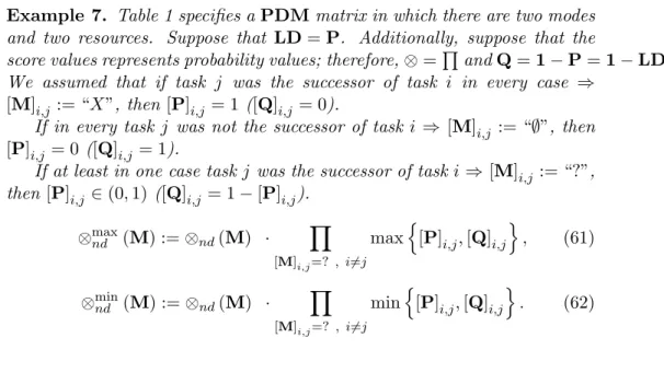
Example 7. Table 1 specifies aPDMmatrix in which there are two modes and two resources. Suppose that LD=P. Additionally, suppose that the score values represents probability values; therefore,⊗=Q

andQ=1−P=1−LD.

We assumed that if task j was the successor of task i in every case ⇒ [M]_i,j := “X”, then [P]_i,j = 1 ([Q]_i,j = 0).

If in every task j was not the successor of task i ⇒ [M]_i,j := “∅”, then [P]_i,j = 0 ([Q]_i,j = 1).

If at least in one case taskj was the successor of taski⇒ [M]_i,j := “?”, then[P]_i,j ∈(0,1) ([Q]_i,j = 1−[P]_i,j).

⊗^max_nd (M) :=⊗_nd(M) · Y

[M]_i,j=? , i6=j

max n

[P]_i,j,[Q]_i,j o

, (61)

⊗^min_nd (M) :=⊗_nd(M) · Y

[M]_i,j=? , i6=j

minn

[P]_i,j,[Q]_i,jo

. (62)

We assumed that [P]_i,j was the relative frequency of task/dependency occurrences. Therefore, the aim of the simulation was to determine the most probable project structure that can be completed given a specified dead- line/budget/resource availability.

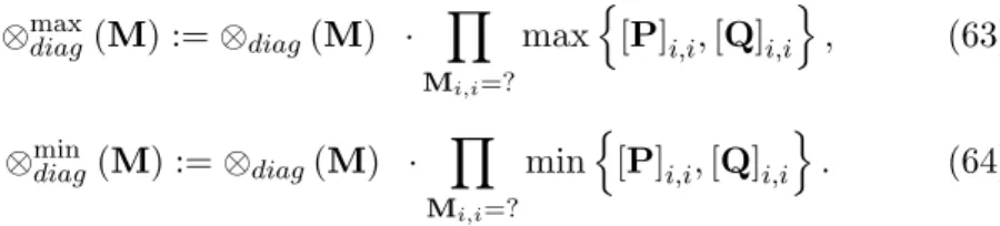
⊗^max_diag(M) :=⊗_diag(M) · Y

Mi,i=?

maxn

[P]_i,i,[Q]_i,io

, (63)

⊗^min_diag(M) :=⊗_diag(M) · Y

Mi,i=?

minn

[P]_i,i,[Q]_i,io

. (64)

Let the durations be in weeks, cost demands be in $1,000 and resource demands be in number of employees. The most-probable project scenario

Table 1: Multi-modal specified PDM

Logic Domain TD CD QD RD

PDM A B C D E tmin tmax cmin cmax qmin qmax r1 min r1 max r2 min r2 max

A 0.8 1.0 0.8 0.2 0.1 4 6 2.4 3.4 0.8 0.9 2.5 4.5 1.6 3.7 B 0.0 1.0 0.0 0.4 0.8 2 3 1.8 2.6 0.7 0.8 3.4 4.2 2.5 4.8 C 0.0 0.0 0.9 0.0 0.2 4 8 9.5 9.9 0.8 0.9 3.8 5.7 1.2 3.5 D 0.0 0.0 0.0 0.4 0.3 9 9 4.2 4.2 0.8 0.8 2.3 2.3 1.4 1.4 E 0.0 0.0 0.0 0.0 0.7 3 4 0.9 1.2 0.7 0.8 3.4 4.7 2.5 6.2

Constraints: 10.0 18.0 0.7 10.0 10.0

contains tasks A,B,C and E, and the probability value of this project sce- nario is ⊗(LD)^max_diag = 0.8 · 1.0 ·0.9 ·(1− 0.4)·0.7 = 0.3024, whereas

⊗(LD)^min_diag= (1−0.8)·1.0·(1−0.9)·0.4·(1−0.7) = 0.0024. The minimal project duration is obtained if all flexible tasks and all flexible dependencies are excluded from this project and all tasks are completed within the shortest possible duration. Since only task2(task B) is a mandatory task, TPTmin = min_j[TD]_2,j = min{2,3} = 2 weeks. This is a global minimum; therefore, there is no way to complete the project in less than 2 weeks. The minimal project cost also occurs if only the mandatory task is completed; however, the cost demands are assumed to be independent of the completion sequences of the tasks. TPC_min = min_j[CD]_2,j = min{1.8,2.6}= 1.8×$1,000 = $1,800.

According to Eqs. (21)-(21), TPQ_max = 1, and the maximum of the re- source demands is minimal when all supplementary tasks are ignored but all flexible dependencies between mandatory tasks are prescribed and the resource demands in the completion modes of mandatory tasks are mini- mal. TPR_min = {3.4; 2.5}. These bounds specify global minima/maxima;

however, if a supplementary task or a flexible dependency is decided to be included in or excluded from the project, and in this manner, we obtain a

restricted matrix, the minimal project cost/durations/resource demands and maximal project quality can be calculated for the restricted matrix.

Remark 3. Since Eqs. (63)–(64) give small values, if there are many tasks, the geometric mean of task scores is calculated and explored. The main advantage of using the geometric mean of task scores instead of multiplying the relative frequencies is that different project scores can be compared.

If M represents the initial hybrid logic plan and M⁰ is the result (final project scenario) of phase one, then

T P S% =⊗_diag(M)% :=



 pn

⊗_diag(M⁰)

n

q⊗^min_diag(M)

−1



×100 (65) denotes the total project score (TPS) performance of project sce- nario M⁰.

TPS%=⊗_diag% ∈ [0,∞]. This value shows us how many times larger the project score is compared to the minimal requirement.

The performance schedules for the remaining parameters are specified as follows (similarly to Eq. 65):

T P Q% :=

T P Q(M,(W)) T P Qmin(M,(W))−1

×100, (66)

T P T% :=

T P Tmax(M,(W)) T P T(M,(W)) −1

×100, (67)

T P C% :=

T P C_max(M,(W)) T P C(M,(W)) −1

×100, (68)

T P R_i% :=

T P R_imax(M,(W)) T P Ri(M,(W)) −1

×100, i= 1,2.., r. (69) Remark 4. Eqs. (65)–(69) are between [0,∞] if the project schedules are feasible. Otherwise, these values are 0.

2.3. The Algorithms 2.3.1. Phase one

We are given the matrix M0 ∈ {X,∅,?}^n×n. Suppose that all the “?”

symbols in the diagonal are in the first σ rows (columns). The algorithm sequentially changes these symbols to either “X” or “∅” inthisorder; such a

change is called astep. These changes are not final, and the original matrix M₀ is also saved. We look for the optimum similarly to a “back-and-forth”

method, saving information in thebuffer B (a set) of possible manners we might investigate later. After replacing as many elements ofM as we can (satisfying Eqs. (42), (43), and (45)), we go back to the cases in whichB has higher scores ⊗_diag than M. (All the possible variations of M₀ form a binary tree of size 2^σ with rootM0.)

Here, M denotes the actual matrix before the next replacement, such that [M]_j,j = “?” ⇐⇒ i ≤ j ≤ σ for some 1 ≤ i ≤ σ, and denote by M[i, i=Y] the matrixafter replacingMi,i toY, whereY ∈ {X,∅}. Before replacing [M]_i,i, we save theother possibility, which we do not follow in the present step, inB. The elements ofB are of the form

b =

i, [M]_1..n,1..n , Y, ⊗^max_diag(M[i, i=Y])

(70)

= (i,−→m, Y,⊗_b), (71)

where i denotes the elements in the diagonal of M that we are replacing,

−

→m =M_1..n,1..nis the actual content of the diagonal ofM(specificallyM_i,i =

“?”), Y ∈ {X,∅} and ⊗_b =⊗^max_diag(M[i, i=Y]) is the“ideal” score that we may achieve by replacing Mi,i with Y.⁶ B may contain several elements with the same ⊗_b value, but at this moment, we do not know which pf these elements can be realized later, i.e., satisfy (42)–(45)

Remark 5. B contains only M[i, i=Y]extensions that have not yet been investigated but fulfill the bounds of (42)–(45). More precisely, for their extension,

C_min(M[i, i=Y],W) ≤ C_c, (72) Tmin(M[i, i=Y],W) ≤ Ct, (73) Qmax(M[i, i=Y],W) ≥ Cq, (74)

⊗^max_diag(M[i, i=Y]) ≥ Cdiag. (75) Remark 6. Before starting step i for 1 < i, at the end of step i−1, we have inserted Y into the i−1-th entry of M. Since we are now ex- tending this configuration, B does not contain the corresponding record b= (i−1,−→m, Y,⊗_b).

6⊗b in (71) denotes a nonnegative real number, and⊗^max_diag was defined in (10).

The algorithm starts a new cycle whenever it goes back to an element ofB and starts to replace “?” from the i=i₀+ 1-th entry of the diagonal.

Problem 1 may have a solution if, for at least one cycle, we are able to stepitoσ (satisfying (42)–(45)). Of course, we store all the in-closures M⁰ of M₀ that were found by the algorithm and may be optimal solutions to Problem 1. If B contains an element b with a higher score than M⁰ has (i.e., ⊗_b > ⊗_diag(M⁰)), then we start a new cycle from b. During this cycle,i cannot be increased to σ,⊗_b =⊗^max_diag(M[i, i=Y]) may fall below

⊗_diag(M), or we might obtain a solution better than M⁰. START Let i0 := 0,i= 1, B:=∅.

GENERAL STEP (1≤i≤σ), Mis the actual matrix. Let bⁱ_X : = i, M1..n,1..n, X, ⊗^max_diag(M[i, i=X])

, (76)

bⁱ_∅ : = i, M1..n,1..n, ∅, ⊗^max_diag(M[i, i=∅])

. (77)

Case i) Neither bⁱ_∅ norbⁱ_X fulfills (72)–(75) andB =∅. Then, STOP since Problem 1 has no solution.

Case ii) Neither bⁱ_∅ nor bⁱ_X fulfills (72)–(75) but B 6=∅. Recall that in Cases i) and ii), B may contain elements of type b = (j,−→m, Y,⊗_b) only if j < i by Note 5 and (70), (71), and (76), (77). In Case ii), choose any elementb∈B such that⊗_b is maximal (inB). Then, reset the diagonal of Maccording to−→m, seti:=j, deletebfrom B, and proceed to the General Step.

Case iii) Exactly one of bⁱ_X or bⁱ_∅ fulfills (72)–(75), say, bⁱ_Y. Let M_i,i:= “Y” and go to Step Increasing i.

Case iv) Both bⁱ_X and bⁱ_∅ fulfill (72)–(75).

If ⊗^max_diag(M[i, i=X])≤ ⊗^max_diag(M[i, i=∅]), then letMi,i := “∅”, B :=

B∪

bⁱ_X , and go to Step Increasing i.

If ⊗^max_diag(M[i, i=X])>⊗^max_diag(M[i, i=∅]), then letMi,i:= “X”, B:=

B∪

bⁱ_∅ , and go to Step Increasing i.

STEP INCREASING(i) Ifi < σ, then leti:=i+ 1 , and go to the General Step. In the casei=σ, go to the Check Step.

CHECK STEP (i=σ) First, save the recent Mwith its⊗_diag(M).

IfB contains an elementb= (i,−→m, Y,⊗_b) such that

⊗_b>⊗_diag(M), (78) then go back to b and start a new cycle, i.e., reset the diagonal of M according to−→m, seti:=j, deleteb from B, and go to the General Step.

END of the Algorithm.

Remark 7. If we want to find all optimal solutions to Problem 1, then replace (78) with

⊗_b ≥ ⊗_diag(M). (79) Of course, we must first save (in an output buffer) the solution(s) we have found thus far. Then, we pick the next element b ∈B in the buffer, reset the diagonal of M according to −→m, set i:= j, delete b from B, and go to the General Step.

We call this algorithm theHybrid Project Ranking algorithm.

Theorem 3. The saved matrices (in the Check Step) of the above algorithm are exactly the optimal solutions to Problem 1. Specifically, there are no saved matrices if and only if (42)–(44) in Problem 1 has no solution at all.

Proof. In each step, the algorithm chooses the best of (at most) two possi- bilities but buffers the other for further investigation. The value⊗_diag(M) for eachMis a sharpupper bound for further continuation ofM. Therefore, all the buffered possibilities with smaller⊗ than those of the finished (and saved) matrices (in the Check Step) could be deleted from the buffer. Since the algorithm checks each remaining element of the buffer (see the Check Step), at the end, we must obtain each optimal solution.

The result of phase one is to find (depending on the meaning of the completion scores and the aggregation functions (see Definition 4)) the most- desirable or most-probable project scenario. The goal of phase two is to find the most-desirable/most-probable project structure within a project scenario. However, the project structure always depends on the result of phase one. Therefore, the “highest”-scoring project structure can be in- terpreted only within a specified project scenario.

2.3.2. Phase two

In phase two, the goal is to find the most-probable or most-desirable project structure within the specified project scenario. The algorithm and most of the notation for phase two are the same as in phase one. We have to determine the “?” symbols off of the diagonal ofM in a fixed (but arbitrary) order. Before each replacement, we save the other possibility in a buffer similarly to (70), checking the conditions corresponding to (47) and (48), such as (72)–(75) corresponded to (42)–(44). In each step, we have to refresh Tmin(M,W) and ⊗_nd(M). The properties of the phase two algorithm can be proven along the lines of Theorem 3 and Subsection 2.3.4.

2.3.3. Phase three

After phase two we obtain a project structure, which represents a traditional resource-constrained time-quality-cost trade-off problem (RC- TQCTP). If there is no feasible solution to the given RC-TQCTP algorithm, we should go back tophase twoand select the next project structure from the buffer.

The result of the RC-TQCTP will produce the optimal solution to the resource-constrained hybrid time-quality-cost trade-off problem.

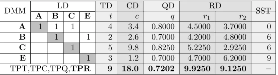
The optimal output matrix is a domain mapping matrix (DMM) (see Table 2), in which flexible dependency and uncertain task completion are excluded or included. Therefore, the logic domain of the output matrix is a DSM.

Table 2: The output matrix of the proposed algorithm if the input is specified by Table 1

LD TD CD QD RD

DMM A B C E t c q r₁ r₂ SST

A 1 1 1 4 3.4 0.8000 4.5000 3.7000 0

B 1 1 2 2.6 0.7000 4.2000 4.8000 6

C 1 5 9.8 0.8250 5.2250 2.9250 6

E 1 3 1.2 0.7000 4.7000 6.2000 9

TPT,TPC,TPQ,TPR 9 18.0 0.7202 9.9250 9.1250 – The optimal output matrix (furthermore, the project schedule matrix) contains one vector of time/cost demands (TD,CD) and one vector of quality parameters (QD). The PSM also contains ann by r submatrix of resource demands (RD) and a vector of scheduled start times (SST).

2.3.4. Algorithmic complexity

Briefly, in phase one, ⊗_diag(M) is calculated and Tmin(M,W) is re- freshed (see Definition 13) such that each cycle is at mostquasilinear, but we have no bounds on thetotal size of the buffer. Similarly, inphase two, we have to calculateTmin(M,W) and ⊗_nd(M), which implies the same upper bound on time as in phase one. Perhaps some extreme counterexamples may cause exponential running time, but practical runs (see Section 3) pro- vide quadratic runs.

In more detail, in general, then^th-largest value can be determined within O(nlogn) computation time (e.g., [22]); however, our decision tree is a spe- cial binary heap in which a quasilinear search algorithm can be specified.

In Section 2.3, we saw that the best project structures can be found within

O(t+d), wheretis the number of supplementary task to be completed and dis the number of flexible task dependencies. If there are no supplementary tasks to be completed, the number of possible project structures depends only on the number of flexible dependencies. If there are dflexible depen- dencies, then there are 2^d possible project plans. The project network can be specified as an NDSM. In case of acyclic project networks, the maximal number of flexible dependency is n(n−1)/2, and in this case, the number of possible project structures is 2^n(n−1)/2.

If there aretsupplementary tasks, then 2^tproject scenarios can be spec- ified. In a special case, ift=nandd=n(n−1)/2, then there are 2ⁿproject scenarios and

n

P

j=0 n j

2^j(j−1)/2 project plans.

The computational demand of the proposed hybrid algorithm with re- spect to the fulfilled PEM=LD of a specified deterministic PEM is O(d) = O(n(n−1)/2)≈O(n²) in the case of a fulfilled upper-triangular NDSM, and the runtimeO(d+t) =O(n+n(n−1)/2)≈O(n²) is similar when consider- ing a fulfilled upper-triangular PEM. For example, whenn= 50, completely filled upper-triangular NDSM and PEM specify 5,78·10³⁶⁸ possible project plans, whereas our algorithm finds a project structure withinO(50²) steps.

However, at the end of the project selection process, where we have a fea- sible project structure, the proposed algorithm has to utilize a RC-TQCTP method. In this case, the complexity of the RC-TQCTP method and the complexity of project selection are multiplied. As (multi-mode) resource- constrained versions of TQCTPs, DTQCTPs and STQCTPs, a stochas- tic version of DTQCTPs, are NP-hard problems. The hybrid versions of these problems, namely, hybrid discrete time-quality-cost trade-off prob- lems (HDTQCTP), hybrid stochastic time-quality-cost trade-off problems (HSTQCTP) and (multi-mode) resource-constrained hybrid time-quality- cost trade-off problems, are also NP-hard problems.

3. Simulation results

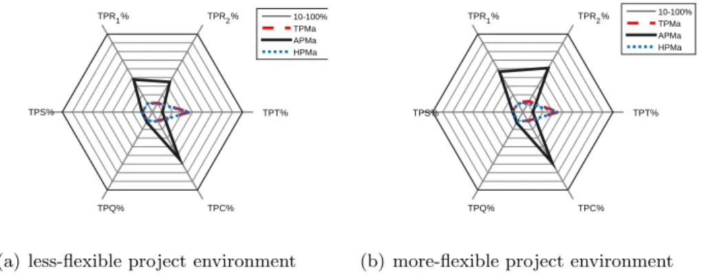
The main goal of the simulation was to compare project scheduling per- formances (see Eqs. (65)–(69)) of the different types of project management approaches.

The first problem was to select an adequate project plan from project database because neither known project generators (such as ProGen [23], RanGen I[24], and II[25]) nor open project data sources (such as MMLIB[26], and PSPLIB[23]) distinguish mandatory and supplementary tasks or con- sider strict and flexible dependencies. Therefore, there are no score values

1

2 3

4

5 7 6 8

9 11 13 10 12

14 15

16

(a) n11 2 (i2= (m−1)/(n−1) = 0.2)

1

2 3

4

5 6

7 8

9

10

11 12

13 15 14

16

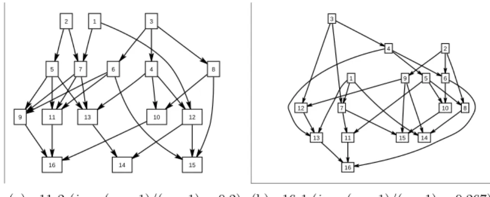
(b) n16 1 (i2 = (m−1)/(n−1) = 0.267) Figure 1: Selected logic network from PSPLIB MRCPSP - n1 dataset

linked to task completion or task dependencies.

The second problem is that the quality parameters are neglected and usually the cost parameters are also missing from the project plans. Addi- tionally, resources are either missing or specified in a discrete multi-mode resource allocation problem, in which there are more than two modes. Nev- ertheless, these project databases have been validated and applied in sev- eral publications for testing and comparing algorithms; therefore, we de- cided to use the logic network, and we extended the project plans with cost, quality, resource and score parameters in the case of the simulation.

Fig. 1 shows the selected logic network from PSPLIB - Multi-Mode Re- source Constrained Project Scheduling Problem (MRCPSP) n1 dataset:

(http://www.om-db.wi.tum.de/psplib/files/n1.mm.zip).

Ref. [27] is specified a real-life project database; however, this database contains only five IT projects, and these projects did not follow the agile approach. In addition, this database did not contain completion modes.

Therefore, project plans were selected from simulation database PSPLIB - MRCPSP - n1 dataset, where the main features of IT projects can be found.

3.1. Simulation database

The aim of the selection and the specification of initial project plans are to meet as much as possible the expectations for (IT) software project plans, especially the features of agile projects:

1. Since Ref. [28] and Ref. [27] showed that software projects usually contain more parallel tasks; therefore, according to the Ref. [28] and

[27], the number of parallel tasks is greater than the number of serial tasks⁷.

2. Projects are usually separated into smaller autonomous sub-projects (sprints) [see, e.g., Ref. 29] that should completed within 2-6 weeks;

therefore, the number of tasks is limited and should not be greater than 20.

3. Contains at least two types of renewable resources (e.g., programmer or tester)

4. Contains two completion modes to apply continuous trade-off methods and in this manner also tests the performance of the hybrid approaches.

The selected n11 2 (see Fig. 1(a)) and n16 1 (see Fig. 1(b)) project plans satisfies criterion 1 (more parallel than serial completion) and criterion 2 (n <20). After selecting logic network, 50-50 project plans are generated for both logic plans n11 2 and n16 1. The minimal value of work hours are set tot_min ∈[20,40] (in work hours) to keep the project duration to within 2-6 weeks. The minimal values of cost demands arecmin ∈[1000,3000] (in

$), which covers the direct costs. The minimal amounts of two types of resources r_min ∈ [3,5] (in terms of number of employees, either testers or programmers) are also specified. At the end, the minimal value of quality parameters q_min ∈ [0.70,0.9] are generated between the specified intervals.

To simulate trade-offs, maximal values were between 110−120% of the minimal values.

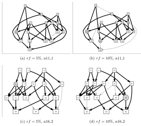
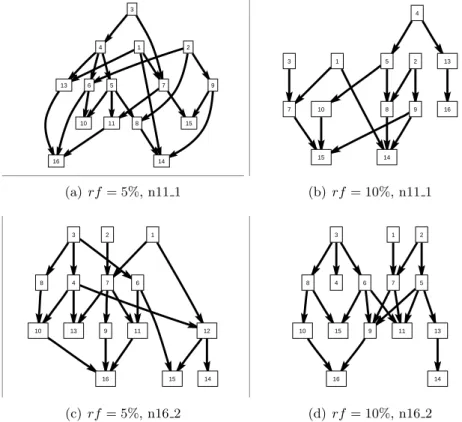
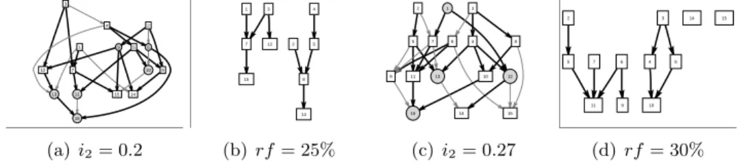
Known project databases (such as ProGen and RanGen I,II) do not dis- tinguish mandatory and supplementary tasks and also do not distinguish fixed and flexible dependencies between two tasks. Consequently, after gen- erating time/cost/resource demands, in our database, the supplementary and mandatory task completions or flexible and strict dependencies are not distinguished. Therefore, in order to simulate flexible environments, two types of datasets are specified. In both cases, first, theratios of flexibil- ity is specified as follows: rf₁ ∈ {5%,10%},rf₂∈ {25%,30%}. This means that in the case of first dataset, 5% and 10%, whereas in the case of dataset 2, 25% and 30% of tasks and dependencies are selected to became supple- mentary tasks or flexible dependencies. In the case of both datasets, it is assumed that the score of including is greater than the score of excluding;

therefore, the score values of supplementary tasks and flexible dependencies

7Following the simulations of Ref. [28],i2 = (m−1)/(n−1)∈[0.2,0.3], wheremis the number stages in a topological ordered network andnis the number of tasks.i2= 1 if all tasks are completed in a serial manner, andi2= 0 if all tasks are completed in parallel.