Ecological Modelling 383 (2018) 41-51.
1
Exploring multiple presence-absence data structures in ecology
2 3
János Podani1,2, Péter Ódor3,8, Simone Fattorini4,5, Giovanni Strona6, Jani Heino7 and Dénes 4
Schmera8,9 5
1 Corresponding author. Department of Plant Systematics, Ecology and Theoretical Biology, 6
Institute of Biology, Eötvös University, Pázmány P. s. 1.c, H-1117 Budapest, Hungary.
7
Email: podani@ludens.elte.hu. ORCID: 0000-0002-1452-1486 8
2 MTA-ELTE-MTM Ecology Research Group, Eötvös University, Pázmány P. s. 1/C, H- 9
1117, Budapest, Hungary 10
3 MTA Centre for Ecological Research, Institute of Ecology and Botany, Alkotmány u. 2-4, 11
H-8237, Vácrátót, Hungary 12
4 Department of Life, Health and Environmental Sciences, University of L’Aquila, L'Aquila, 13
Italy 14
5 CE3C – Centre for Ecology, Evolution and Environmental Changes/Azorean Biodiversity 15
Group and University of Azores, Angra do Heroísmo, Portugal 16
6 European Commission, Joint Research Centre, Directorate D - Sustainable Resources – Bio- 17
Economy Unit, Via Enrico Fermi 274 9, 21027 Ispra (VA), Italy 18
7 Finnish Environment Institute, Natural Environment Centre, Biodiversity, Paavo Havaksen 19
Tie 3, FIN-90570 Oulu, Finland 20
8 MTA Centre for Ecological Research, GINOP Sustainable Ecosystem Group, Klebelsberg 21
K. u. 3, H-8237 Tihany, Hungary 22
9 MTA Centre for Ecological Research, Balaton Limnological Institute, Klebelsberg K. u. 3, 23
H-3237 Tihany, Hungary 24
25
Abstract 26
Ecological studies may produce presence-absence data sets for different taxonomic groups, 27
with varying spatial resolution and temporal coverage. Comparison of these data is needed to 28
extract meaningful information on the background ecological factors explaining community 29
patterns, to improve our understanding of how beta diversity and its components vary among 30
communities and biogeographical regions, and to reveal their possible implications for 31
biodiversity conservation. A methodological difficulty is that the number of sampling units 32
may be unequal: no method has been designed as yet to compare data matrices in such cases.
33
The problem is solved by converting presence-absence data matrices to simplex plots based 34
on the decomposition of Jaccard dissimilarity into species replacement and richness 35
difference fractions used together with the complementary similarity function. Pairs of 36
simplex plots representing different data matrices are then compared by quantifying, for each 37
of them, the relative frequency of points in small, pre-defined subregions of the simplex, and 38
then calculating a divergence function between the two frequency distributions. Given more 39
than two data matrices, classification and ordination techniques may be used to obtain a 40
synthetic and informative picture of metacommunity structure.
41
We demonstrate the potential of our data analytical model by applying it to different case 42
studies spanning different spatial scales and taxonomic levels (Mediterranean Island faunas;
43
Finnish stream macroinvertebrate assemblages; Hungarian forest assemblages), and to a study 44
of temporal changes in small islands (insect fauna in Florida). We conclude that, by 45
accounting for various structural aspects simultaneously, the method permits a thorough 46
ecological interpretation of presence-absence data. Furthermore, the examples illustrate 47
succinctly how similarity, beta diversity and two of its additive components, species 48
replacement and richness difference influence presence-absence patterns under different 49
conditions.
50
Keywords: Beta diversity; Classification; Comparison; Ordination; Similarity; Simplex 51
diagram 52
53
1. Introduction 54
Community data derived from field surveys have been routinely summarized in form of 55
presence-absence matrices, with species (or other taxa) as rows and study objects (e.g., sites, 56
plots, localities, etc.) as columns. A given study may produce two or more data matrices from 57
the same region which differ from one another in taxonomic coverage, spatial resolution, the 58
time of sampling, or any other ecologically meaningful factor. By definition, a meta-analysis 59
attempting to summarize community level information from various and independent sources 60
is also concerned with several data matrices. In all these cases, one is faced with the 61
fundamental problem of comparing the inherent structure of data matrices with 62
heterogeneous origin and properties. By structured presence-absence data we refer here to a 63
matrix containing 0-s and 1-s which deviates from a random arrangement of scores by having, 64
for example, any tendency of grouping, trends, or nestedness. These features are inherent, 65
thanks to their independence from the actual ordering of rows and columns (see Podani &
66
Schmera 2011). Such comparisons are essential to understand variations in beta diversity 67
among communities and biogeographical regions, the ecological factors explaining these 68
patterns, and their possible implications for biodiversity conservation. One possibility to 69
tackle these issues is to perform classification or ordination on each data matrix and then to 70
compare the resulting scatter plots, dendrograms or partitions. However, standard procedures 71
available for this purpose can only be applied to cases in which the number of study objects is 72
the same in all the data sets under evaluation (Podani 2000). The other way to proceed is to 73
compare the data matrices directly, without multivariate analysis, but this methodology – in 74
addition to equality in the number of objects – requires identical number of species as well.
75
(Hubert & Golledge 1982; Zani 1986). That is, no universally applicable method has been 76
developed as yet to compare the structure of data matrices that are unequal in size.
77
As a possible solution to this problem, we suggest a new analytical model that makes it 78
possible to investigate multiple, heterogeneous datasets in a single framework. Essentially, the 79
approach is based on the decomposition of Jaccard dissimilarities between pairs of objects 80
into two additive components, namely species replacement (R) and richness difference (D), 81
which, together with the complementary Jaccard similarity (S), are used to represent data 82
structure as a point cloud in a ternary plot called SDR-simplex (Podani & Schmera 2011;
83
Carvalho et al. 2012). Point clouds representing different data structures can then be 84
compared on the basis of the relative frequencies of points (object pairs) in pre-defined 85
subsections of the ternary plot. Since calculation of a frequency distribution is involved, we 86
shall refer to this strategy as the indirect comparison of simplexes.
87
We suggest that the approach is equally useful to situations where the matrices to be 88
compared represent the same set of objects (for example, when a given set of objects is 89
surveyed for different organism groups, or when a taxonomic group is examined in the same 90
sites several times to monitor temporal changes of community composition), even though in 91
those cases comparisons of ordinations and classifications could also work. This is because 92
decomposition of dissimilarity into additive terms allows separating the effect of major 93
ecological driving forces – a possibility not available otherwise. Now, the simplex plots need 94
not be partitioned; the shapes of point clouds can be directly compared by measuring the shift 95
of the corresponding points in the two configurations.
96
Both indirect and direct comparisons may be performed on all possible pairs of matrices in a 97
multiple dataset, yielding a dissimilarity matrix of SDR simplexes that can be then used in 98
further analyses, such as classifications and ordinations. We emphasize here that this meta- 99
analysis approach is more suited to exploratory analysis rather than to hypothesis-testing. In 100
this paper, we describe in detail the technical aspects of our method, and illustrate its potential 101
in ecological research, by reporting results for both artificial examples and empirical case 102
studies.
103 104
2. Computational steps 105
2.1 The SDR-simplex 106
Jaccard's (1901) similarity coefficient is one of the oldest and most commonly used 107
resemblance functions, computed for any two objects j and k as:
108
sjk = a / (a+b+c), (1)
109
where a is the number of species occurring in both j and k, while b and c correspond to the 110
number of species exclusive, respectively, to j and k. Its complement, Jaccard dissimilarity, is 111
computed as:
112
jk = 1 – sjk = (b+c) / (a+b+c). (2)
113
Dissimilarity can be partitioned into two additive fractions (Podani & Schmera 2011;
114
Carvalho et al. 2012):
115
jk = djk + rjk = | b–c | / (a+b+c) + 2min{b,c} / (a+b+c), (3) 116
where djk = | b–c | / (a+b+c) is the relative richness difference, while rjk = 2min{b,c} / (a+b+c) 117
is the relative species replacement with respect to objects j and k. In the latter, the numerator 118
is the maximum fraction of the so-called species turnover which is equally shared by j and k.
119
Since sjk + djk + rjk = 1, these three quantities may be used to define the relative position of the 120
point representing object pair jk with respect to the three vertices (S–Similarity, D–richness 121
Difference and R–species Replacement) of an equilateral triangle, the so-called SDR-simplex 122
diagram (Podani & Schmera 2011). In the SDR-simplex, the distance of each point from a 123
given vertex is inversely proportional to the corresponding fraction, that is, S, D or R. Similar 124
ternary plots have been used in ecology as illustrations of C-S-R strategies of plants (Grime 125
1977), of feeding habits of fish (Fig. 6.9 in Stoffels 2013), and are even more widely used in 126
population genetics (commonly referred to as “de Finetti diagram”) to represent the genotype 127
frequencies of diploid populations for a biallelic locus (Edwards 2000), and in geology to 128
classify rocks and minerals on the basis of their fractional composition (Streckeisen 1976).
129
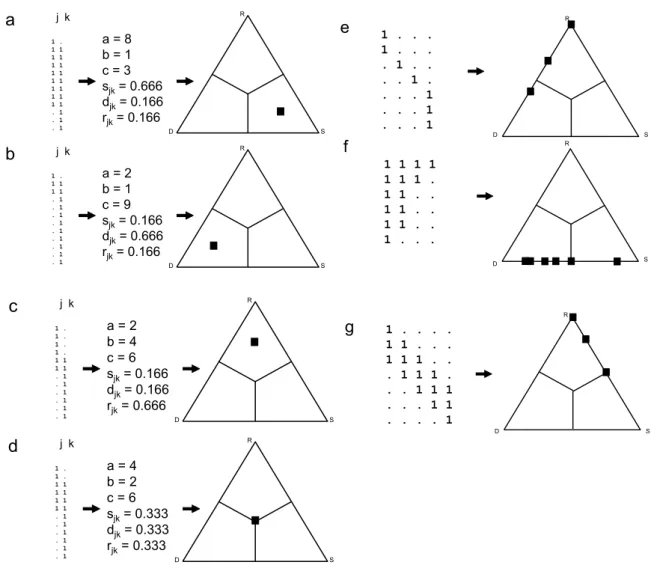
Let us first demonstrate the procedure for a pair of hypothetical objects j and k containing a 130
total of 12 species with different nonzero values of a, b and c. If the objects have many 131
species in common (a = 8), and species replacement and richness difference are equal 132
(2min{b,c} =| b–c | = 2), then the point representing this pair of objects in the ternary plot is 133
positioned close to the S vertex, and with equal distance from D and R (Fig. 1a). If richness 134
difference is high (| b–c | = 9) and similarity and replacement are the same (a = 2min{b,c} = 135
2), then the point moves close to the D vertex (Fig. 1b). Analogously, if species replacement 136
is the dominating phenomenon, with 4 species being replaced by other 4 (2min{b,c} = 8), and 137
the two objects sharing only 2 species, with a richness difference of 2 (a = | b–c | = 2), the 138
point representing j,k in the ternary plot is positioned close to the R vertex, and with equal 139
distance from D and S (Fig. 1c). When the three components are equal (a = 2min{b,c} = | b–c|
140
= 4), the corresponding point will fall onto the center of the triangle (Fig. 1d).
141
In a data matrix X containing m objects, the possible number of pairwise comparisons would 142
be w = (m2 – m) / 2, each corresponding to a point in the simplex. Notably, the shape of the 143
point cloud in a simplex is unaffected by the actual arrangement of rows and columns in the 144
matrix. “Extreme” structural patterns produce clear distributions of points in the triangle. If 145
compositional similarity is high for all pairs, the point cloud will be near the S corner. When 146
the objects have extreme richness difference, with low replacement and similarity, the points 147
will be close to the D vertex. In cases when richness is similar but similarity is low, the points 148
will be in the upper third of the diagram. These cases are extensions of the two-object 149
situations explained above, and are not illustrated. However, there are further noted examples 150
in which two of the three components contribute approximately equally to data structure, 151
whereas the third is zero. Maximum beta diversity (anti-nestedness) in the data (with sjk = 0 152
for all j k), makes all points fall onto the left (D-R) side of the triangle (Fig. 1e), while 153
maximum nestedness of objects (with rjk = 0 for all pairs) forces all points to the bottom (D-S) 154
side (Fig. 1f). In case of a perfect gradient (when the species richness is constant, the same 155
number of species are lost and gained at each sampled step along that gradient, and djk = 0 for 156
all pairs) all points are distributed on the S-R side (Fig. 1g). See Podani & Schmera (2011), 157
for further examples of structural patterns and their simplex representations. The position of 158
the centroid of the point cloud (calculated as the means of the sjk, djk and rjk values) will be 159
used in a synthetic measure to compare the structure of comparable plots. Furthermore, these 160
means multiplied by 100 quantify the percentage contributions of the three fractions to 161
community pattern. In addition to these contributions, it is also useful to consider the 162
percentage of presence scores in the data matrix, i.e., matrix fill, denoted here by q.
163
test
D
R
S
1 . . . 1 . . . . 1 . . . . 1 . . . . 1 . . . 1 . . . 1
e
test
D S
1 1 1 1 1 1 1 . 1 1 . . 1 1 . . 1 1 . . 1 . . .
f R
test
j k
1 . 1 1 1 1 1 1 1 1 1 1 1 1 1 1 1 1 . 1 . 1 . 1
test
D
R
S
a = 8 b = 1 c = 3 sjk= 0.666 djk= 0.166 rjk= 0.166
a
j k
1 . 1 1 1 1 . 1 . 1 . 1 . 1 . 1 . 1 . 1 . 1
. 1 D
R
S
a = 2 b = 1 c = 9 sjk= 0.166 djk= 0.666 rjk= 0.166
b
j k
1 . 1 . 1 . 1 . 1 1 1 1 . 1 . 1 . 1 . 1 . 1 . 1
test
D
R
S
a = 2 b = 4 c = 6 sjk= 0.166 djk= 0.166 rjk= 0.666
c
j k
1 . 1 . 1 1 1 1 1 1 1 1 . 1 . 1 . 1 . 1 . 1 . 1
test
D
R
S
a = 4 b = 2 c = 6 sjk= 0.333 djk= 0.333 rjk= 0.333
d
g
D
R
S
1 . . . . 1 1 . . . 1 1 1 . . . 1 1 1 . . . 1 1 1 . . . 1 1 . . . . 1
164 165
Fig. 1. (a-d) The three fractions and the position of the corresponding point in the ternary plot 166
for a pair of artificial objects for various values of a, b and c. (e) A simple case of maximum 167
beta diversity (anti-nestedness) for 4 objects (columns) and its representation in a ternary plot.
168
(f) A case of maximum nestedness for 4 objects and the corresponding SDR-simplex. (g) 169
Perfect gradient for 5 objects as is depicted by the simplex plot. Note that the number of 170
object pairs, therefore the number of symbols is six in (e)-(f) and 10 in (g), but many of them 171
overlap in the plot.
172 173
2.2 Indirect comparison of two SDR-simplexes for different sets of objects 174
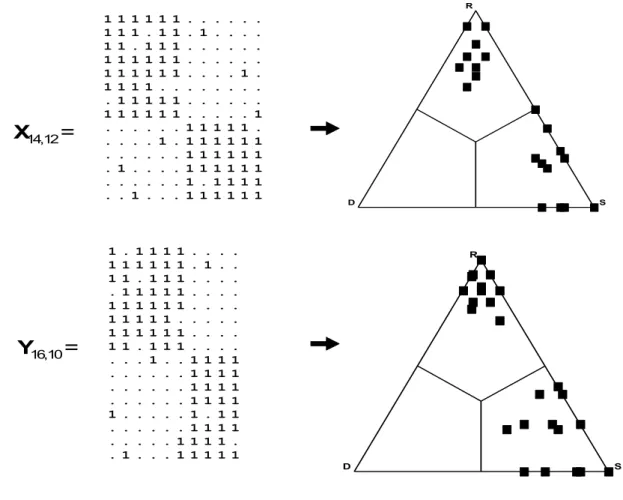
Assume that we have another data matrix, Y, with p objects. Although p can differ 175
considerably from m, the two corresponding point clouds in the ternary plots may have 176
similar appearance, notwithstanding that the number of constituting points (w versus z = [p2– 177
p]/2) will be clearly different. Similarities in the shape of point clouds should reflect similar 178
structure in the two data matrices, as demonstrated by the artificial examples in Figure 2. In 179
these sample matrices, the species and the objects are co-distributed to form an almost perfect 180
modular pattern (with, in both cases, two large and clearly identifiable modules manifested as 181
blocks of contiguous “1” values in the matrix). Converting the two data matrices into SDR- 182
simplex triangles makes their structural similarity obvious. For both matrices, one set of 183
points corresponds to within-block (near the S vertex) comparisons, while the other set of 184
points represents between-block (near the R vertex) comparisons.
185
Although the visual examination of SDR simplexes is appealing and immediate, it is clear 186
how simplexes’ geometrical properties offer a possible solution to the problem of comparing 187
heterogeneous datasets, overcoming the difficulties posed by matrix-level comparisons. The 188
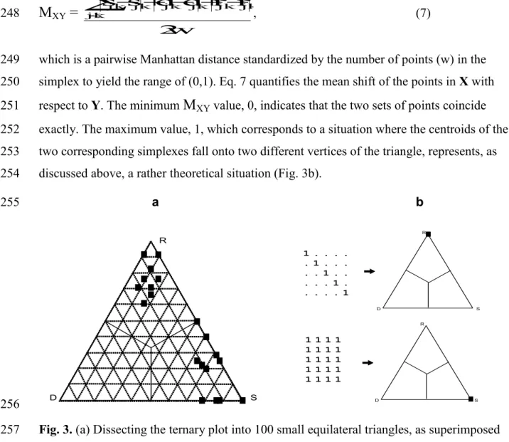
spatial position of point sets AX and BY within the corresponding triangle may be simplified 189
into the relative frequency distributions FX and GY, respectively, following the dissection of 190
each triangle into small equilateral triangles identical in size, as shown in Fig. 3 (where 100 191
small triangles are used). Each value fi in FX is obtained as the number of points falling into 192
small triangle i, divided by w, in the simplex diagram corresponding to X. The problem with 193
points falling right onto the sides of small triangles is resolved in a systematic way (see 194
Appendix S1 in Supplementary Information, for algorithmic details). Values in GY are 195
derived in the same manner, dividing all gi-s by z. Then, the divergence between the two 196
distributions will provide the desired quantity:
197
EXY =
100
1 i
i i
z g w
f ,
(4)
198
that is the sum of the absolute differences between the corresponding relative frequencies over 199
the 100 small triangles. Its maximum is 2, obtained when the two point clouds do not overlap, 200
therefore EXY may be divided by 2 to obtain a dissimilarity with a range of (0,1) 201
E’XY =
100
1 i
i i
z g w f 2
1
.
(5)202
Although the above calculation may seem to provide a straightforward solution, the same 203
E’XY value of 1 may result for radically different situations: in fact, the maximum possible 204
difference between two sets is recorded both when the point sets AX and BY fall into close, but 205
not overlapping positions, or when they fall right onto two different vertices of the triangle.
206
However, it should be considered that the D vertex is usually not occupied by actual data 207
(because it corresponds to localities with no species, which, apart from few exceptions, are 208
normally excluded from meta-community matrices). Thus, the maximum E’XY value should 209
more logically correspond to a situation where AX corresponds to perfect species replacement 210
(all points fall on the R vertex), and BY depicts complete similarity (all points coincide with 211
the S vertex, see Fig. 3b). In the triangular representation, the distance between these vertices, 212
that is, the maximum distance within the plot, is scaled appropriately to 2 = 213
.
214
To tackle this issue, we suggest including the distance between the centroids of point sets AX
215
and BY, abbreviated ascXY, as a weighting factor in Eq. 5. The weighting factor is defined to 216
be tXY = 1 when the centroids coincide, and tXY = 1 + cXY otherwise. Since weighting 217
influences the maximum, it is advisable to rescale the quantity into the unit range using the 218
maximum centroid distance, i.e., 2 to obtain a measure of dissimilarity between two simplex 219
configurations:
220
XY =
) 2 1 ( 2
z g w ) f c 1
( 100
1 i
i XY i
(6)
221
In this, the maximum is 1, achieved only if the centroids fall onto the vertices, that is, in the 222
unique situation described above. The minimum value, 0, is obtained when the centroids of 223
the two point clouds coincide, and the relative frequency distributions FX and GY are in 224
perfect agreement. This does not imply, however, that zero reflects complete identity of the 225
two data structures being compared. Note that the two matrices need not be equal in size to 226
yield XY = 0, and that, additionally, the same result can be obtained when the differences 227
between the two simplex configurations are small enough to produce identical relative 228
frequencies. For these reasons, our measure is close to what the mathematicians call 229
pseudometric, or semi-distance (Vialar 2016, p. 312). For the two matrices in Fig. 2, we 230
obtain XY = 0.19.
231 232
1 1 1 1 1 1 . . . . 1 1 1 . 1 1 . 1 . . . . 1 1 . 1 1 1 . . . 1 1 1 1 1 1 . . . . 1 1 1 1 1 1 . . . . 1 . 1 1 1 1 . . . . . 1 1 1 1 1 . . . . 1 1 1 1 1 1 . . . 1 . . . 1 1 1 1 1 . . . . . 1 . 1 1 1 1 1 1 . . . 1 1 1 1 1 1 . 1 . . . . 1 1 1 1 1 1 . . . 1 . 1 1 1 1 . . 1 . . . 1 1 1 1 1 1
1 . 1 1 1 1 . . . . 1 1 1 1 1 1 . 1 . . 1 1 . 1 1 1 . . . . . 1 1 1 1 1 . . . . 1 1 1 1 1 1 . . . . 1 1 1 1 1 . . . . . 1 1 1 1 1 1 . . . . 1 1 . 1 1 1 . . . . . . . 1 . . 1 1 1 1 . . . 1 1 1 1 . . . 1 1 1 1 . . . 1 1 1 1 1 . . . 1 . 1 1 . . . 1 1 1 1 . . . 1 1 1 1 . . 1 . . . 1 1 1 1 1
X14,12 =
Y16,10 =
D
R
S
D
R
S
233 234
Fig. 2. Two matrices of different size with similar data structure, and the corresponding SDR- 235
simplex diagrams.
236 237
2.3 Comparison of two data matrices for the same set of objects 238
A carefully designed study may provide several matrices representing, for example, the same 239
meta-community sampled at different times (i.e., sequential snapshots of the same matrix) or 240
the same set of objects sampled for different sets of organisms. In such cases, the above 241
method may be considerably simplified into direct comparison, without dissecting the ternary 242
plots into small triangles. Since every member of the set AX has its counterpart in GY, we can 243
calculate the relative shift in position between each pair of points in the ternary plot. A 244
straightforward solution to measure the shift is offered by the additive fractions of the Jaccard 245
coefficient. The desired measure takes the following form, where upper indices refer to the 246
two matrices being compared:
247
M
XY=
w 2
r r d d s s
k j
Y jk X jk Y jk X jk Y jk X
jk
, (7)
248
which is a pairwise Manhattan distance standardized by the number of points (w) in the 249
simplex to yield the range of (0,1). Eq. 7 quantifies the mean shift of the points in X with 250
respect to Y. The minimum
M
XY value, 0, indicates that the two sets of points coincide 251exactly. The maximum value, 1, which corresponds to a situation where the centroids of the 252
two corresponding simplexes fall onto two different vertices of the triangle, represents, as 253
discussed above, a rather theoretical situation (Fig. 3b).
254
a b
255
2
1
3S R
D D
R
S D
R
S
1 . . . . . 1 . . . . . 1 . . . . . 1 . . . . . 1
1 1 1 1 1 1 1 1 1 1 1 1 1 1 1 1 1 1 1 1
256
Fig. 3. (a) Dissecting the ternary plot into 100 small equilateral triangles, as superimposed 257
onto the SDR-simplex on top in Fig. 2. (b) The rather theoretical situation when the two 258
simplexes maximally differ: the upper one representing pure species replacement while the 259
other corresponding to complete overall similarity.
260 261
2.4 Meta analysis and computer programs 262
If the study involves the comparison of k data matrices in every possible pair, a natural 263
question is how to extract new information from the dissimilarity matrix of simplexes in order 264
to explain underlying factors affecting ecological or biogeographical patterns in the starting 265
datasets. That is, the next step is a sort of meta-analysis. The most straightforward approach to 266
the issue is multivariate exploration, i.e., the application of some methods of numerical 267
classification and ordination (Podani 2000). In the present case studies, we performed group 268
average clustering (UPGMA, Sneath & Sokal 1973) and metric multidimensional scaling (or 269
principal coordinates analysis, PCoA, Gower 1966), two procedures routinely used in 270
biological data analysis. Interpretation of PCoA plots is enhanced by a posteriori 271
superposition of arrows representing the three simplex fractions and matrix fill. The 272
coordinates of these arrows are the correlations with the axes themselves, rescaled arbitrarily 273
to fit the plotted area. Note that despite their similarity in graphical appearance, these 274
ordination diagrams cannot be interpreted as conventional biplots.
275
The between-simplex dissimilarities were calculated by the SDR-DIST stand-alone WIN 276
application written by the first author. Numerical results for the SDR simplex diagrams were 277
prepared by program SDRSimplex (Podani & Schmera 2011). Cluster analysis and 278
multidimensional scaling were performed and the simplex plots were drawn by using the 279
SYN-TAX 2000 package (Podani 2001). All of these programs and their documentation can 280
be downloaded free of charge from http://ramet.elte.hu/~podani. In addition, a thoroughly 281
commented R script including all the functions needed to replicate in full the analysis 282
performed in the present paper is provided in Appendix S3.
283 284
3. Case studies 285
We present here the main results for four different case studies, reporting a full description of 286
datasets and a more thorough interpretation of results in Supplementary Information.
287 288
3.1 Biogeography of the central Aegean Islands.
289
We compiled 12 presence-absence matrices using published distributional data (see Appendix 290
S2) for land snails, isopods, chilopods (centipedes), tenebrionid beetles, butterflies and 291
reptiles from two island groups (Anatolian and Cycladic) in the Aegean Sea (east 292
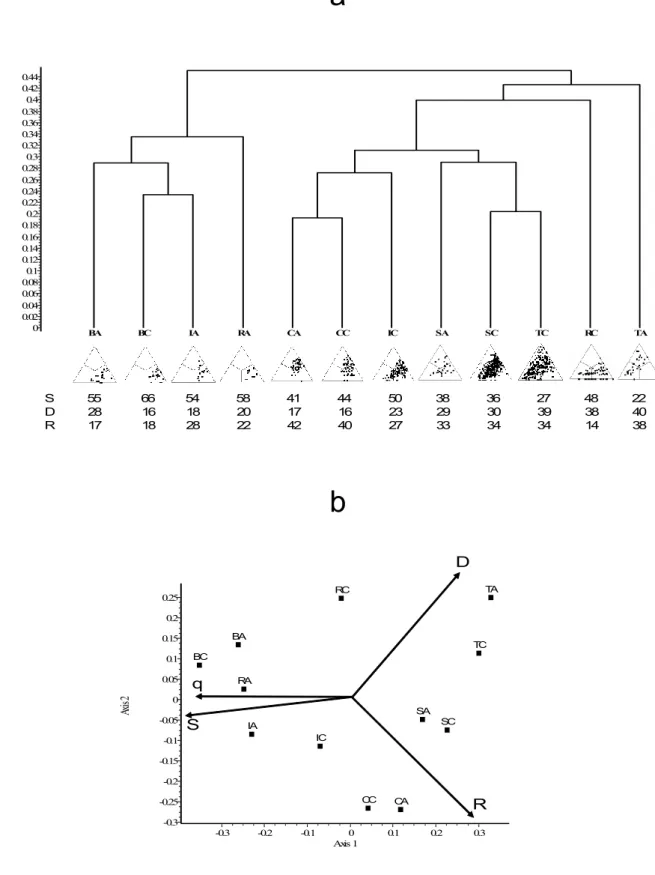
Mediterranean). Exploratory analysis of the 12 simplex diagrams via hierarchical 293
classification identifies two large clusters (Fig. 4a). The group in the left includes matrices 294
with the highest overall similarity (and the lowest beta diversity), namely butterflies in both 295
island groups, and isopods and reptiles in the Anatolian islands. In the right group, data 296
matrices have higher beta diversity (both data matrices for centipedes; snails and tenebrionids, 297
and the isopods and reptiles in the Cyclades).
298
a
299
Dissimilarity
0.44 0.42 0.4 0.38 0.36 0.34 0.32 0.3 0.28 0.26 0.24 0.22 0.2 0.18 0.16 0.14 0.12 0.1 0.08 0.06 0.04 0.02
0 BA BC IA RA CA CC IC SA SC TC RC TA
S 55 66 54 58 41 44 50 38 36 27 48 22 D 28 16 18 20 17 16 23 29 30 39 38 40 R 17 18 28 22 42 40 27 33 34 34 14 38
300
b
301
Axis 10 0.1 0.2 0.3
-0.1 -0.2 -0.3
Axis 2
0.25 0.2 0.15 0.1 0.05 0 -0.05 -0.1 -0.15 -0.2 -0.25 -0.3
BC BA
RA
IA
IC RC
CC CA SA
SC TC
TA
S
R D
q
302
Fig. 4. (a) UPGMA dendrogram for the Mediterranean islands example. The SDR-simplex 303
diagrams are shown in miniature under each label together with the percentage contributions 304
from the S (right corner), D (left corner) and R (top corner) fractions. (b) PCoA ordination of 305
faunas; scaling of arrows: 0.4 = unit correlation. Abbreviations as in Table 1.
306
307
Both the Anatolian and the Cycladic butterfly faunas are characterized by high species 308
distributional overlaps, possibly related to high species dispersal ability, which may promote 309
butterfly persistence in most islands of both archipelagos. A similar pattern and interpretation 310
applies to reptiles in the Anatolian islands. Conversely, reptiles’ tendency for nestedness 311
(S+D=86%, the highest in this case study) in the Cyclades could possibly be a result of local 312
extinctions, as reconstructed by Foufopoulos & Ives (1999) and Foufopoulos et al. (2011).
313
Isopods exhibit high species similarity in the Anatolian islands as well, but not in the 314
Cyclades. The relative placement of Anatolian and Cycladic isopods in the dendrogram and in 315
the ordination analysis reflects the similar positions of their centroids in the SDR plots (for IA 316
– Anatolian Isopods: 54%, 18%, 28%, for IC – Cycladic Isopods: 50%, 23%, 27%). However, 317
the larger variance of points in the Cyclades data prevents IA and IC from clustering together.
318
Many species are common to most islands in both archipelagos, as reflected by many points 319
falling into the S section of the simplex, possibly corroborating the idea that isopods are not 320
as poor dispersers as generally thought (Tajoský et al. 2012). The higher level of nestedness 321
in the Cyclades could be due to isopod distribution in a larger number of islands (16 islands, 322
vs. 6 in the Anatolian group) which, in turn, may reflect potential interspecific differences in 323
dispersal ability.
324
The distributional pattern of centipedes is highly consistent in the two island groups, with 325
most communities tending towards richness agreement and comparable levels of species 326
replacement and similarity, possibly due to centipedes’ high dispersal ability (Simaiakis &
327
Martínez-Morales 2010). Ternary plots reveal similar patterns for land snails in the two 328
archipelagos, with most points scattered around the center, indicating randomness. This may 329
reflect a combination of high population abundances (which may compensate for low 330
dispersal ability), similarities in the interspecific dispersal abilities, and a certain degree of 331
randomness in dispersal events.
332
Both ternary plots indicate a situation with large overlap between tenebrionid species 333
composition within certain island groups, and large differences between the two island 334
groups. These differences cannot be due to bias in sampling records, because occurrences of 335
tenebrionids on the Aegean islands are well known (Pitta et al. 2017). Rather, this pattern may 336
reflect a combination of current rare, overseas, long-distance dispersal and past colonization 337
via land-bridges.
338
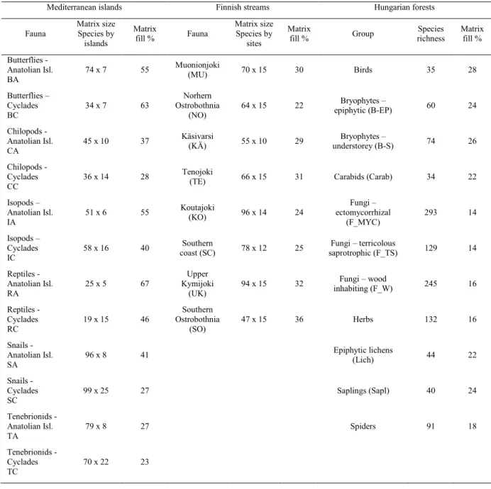
Table 1. Main features and abbreviations for data sets used in case studies.
339
Mediterranean islands Finnish streams Hungarian forests
Fauna
Matrix size Species by islands
Matrix
fill % Fauna
Matrix size Species by
sites
Matrix
fill % Group Species
richness Matrix fill % Butterflies -
Anatolian Isl.
BA
74 x 7 55 Muonionjoki
(MU) 70 x 15 30 Birds 35 28
Butterflies – Cyclades BC
34 x 7 63
Norhern Ostrobothnia
(NO)
64 x 15 22 Bryophytes –
epiphytic (B-EP) 60 24
Chilopods - Anatolian Isl.
CA 45 x 10 37 Käsivarsi
(KÄ) 55 x 10 29 Bryophytes –
understorey (B-S) 74 26
Chilopods - Cyclades CC
36 x 14 28 Tenojoki
(TE) 66 x 15 31 Carabids (Carab) 34 22
Isopods – Anatolian Isl.
IA
51 x 6 55 Koutajoki
(KO) 96 x 14 24
Fungi – ectomycorrhizal
(F_MYC)
293 14
Isopods – Cyclades IC
58 x 16 40 Southern
coast (SC) 78 x 12 25 Fungi – terricolous
saprotrophic (F_TS) 129 14 Reptiles -
Anatolian Isl.
RA
25 x 5 67
Upper Kymijoki
(UK)
94 x 15 32 Fungi – wood
inhabiting (F_W) 245 16
Reptiles - Cyclades
RC 19 x 15 46
Southern Ostrobothnia
(SO) 47 x 15 36 Herbs 132 16
Snails - Anatolian Isl.
SA
96 x 8 41 Epiphytic lichens
(Lich) 44 22
Snails - Cyclades SC
99 x 25 27 Saplings (Sapl) 40 24
Tenebrionids - Anatolian Isl.
TA
79 x 8 27 Spiders 91 18
Tenebrionids - Cyclades TC
70 x 22 23
340
3.2 The distribution of stream macroinvertebrates in eight regions in Finland.
341
Previous studies on northern streams’ macroinvertebrate communities revealed significant 342
regional differences in species composition and richness (Heino et al. 2002, 2003), evidence 343
of community assembly processes (Heino et al. 2015a), and a strong latitudinal variation in 344
community composition (Sandin 2003), possibly driven by climatic and environmental 345
factors. Here we applied our innovative analytical framework to show how such 346
macroecological patterns can be easily identified (and synthesized) by the SDR approach.
347
We compiled 8 data matrices summarizing the macroinvertebrate species composition in all 348
the streams in eight northern Finnish regions (for details, see Table 1 and Appendix S2). Like 349
in the previous case study, we compared indirectly every possible pair of simplexes, and then 350
we used the resulting dissimilarity matrix to perform an UPGMA cluster analysis and a 351
PCoA.
352
The dendrogram (Fig. 5a) splits the regions into two major clusters of equal size: the left 353
cluster is characterized by relatively high similarity (35-44%) and by species replacement (36- 354
48%) much higher than richness difference (15-20%). This pattern corresponds in the 355
simplexes as points scattered around the centroid, and close to the right edge (richness 356
agreement, S+R edge). This indicates that high richness differences between streams are rare 357
within each region of this cluster. Although the position of the simplex centroid of Southern 358
Ostrobothnia (SO) is close to that of Tenojoki (TE), the point cloud of the first one appears 359
much more elongated, with some pairs exhibiting complete nestedness (on the bottom edge).
360
Data matrices in the other (right) cluster have a much lower tendency for similarity (23-27%), 361
with the R fraction dominating again beta diversity – with the exception of Northern 362
Ostrobothnia (NO), where D and R have fairly equal contribution. In these cases, the point 363
cloud moves closer to the beta diversity (left) edge of the ternary plot. The point cloud is most 364
scattered for Northern Ostrobothnia (NO), reflecting the very high variability in species 365
richness among streams in the region.
366
The ordination along axes 1-2 (accounting for 34% and 18% of variance, respectively) 367
confirms the classification results, with a clear separation between the two clusters on the first 368
axis. This is essentially an S versus beta diversity axis (r1S = –0.99), with high correlations 369
with matrix fill (rqS = 0.89, r1q = –0.87). The vertical axis corresponds to an increasing 370
contrast between the two fractions of beta diversity. On the bottom (Northern Ostrobothnia, 371
NO) contrast is low, i.e., D and R are similar, whereas on the top (Käsivarsi, KÄ) contrast is 372
high, with species replacement (R) being three times higher than richness difference. This is 373
also shown by the relatively high product moment correlation of 2nd axis scores with D (r2D = 374
–0.88) and R (r2R = 0.72).
375
a
376
S 37 37 35 44 26 27 26 23 D 17 19 15 20 35 16 22 24 R 46 43 48 36 39 56 52 53
Dissimilarity
0.3 0.28 0.26 0.24 0.22 0.2 0.18 0.16 0.14 0.12 0.1 0.08 0.06 0.04 0.02
0 MU TE UK SO NO KÄ KO SC
377
b
378
S
D R q
Axis 1
0.2 0.1 0 -0.1 -0.2 -0.3
Axis 2
0.25 0.2 0.15 0.1 0.05 0 -0.05 -0.1 -0.15 -0.2 -0.25 -0.3
SO
TE MU UK
NO KÄ
KO
S SC
D R q
379
Fig. 5. (a) UPGMA dendrogram for the Finnish stream macroinvertebrates example. The 380
SDR-simplex diagrams are shown in miniature under each label together with the percentage 381
contributions from the S (right corner), D (left corner) and R (top corner) fractions, (b) PCoA 382
ordination; scaling of arrows: 0.3 = unit correlation. Abbreviations as in Table 1.
383
384
Overall, the eight regions exhibited a fair similarity in metacommunity structure, mostly 385
driven by between-stream similarity. Contrary to our expectation, however, we did not find 386
strong evidence for latitudinal gradients in the S, D or R components. This finding, however, 387
is in line with studies focusing on regional and local richness patterns in Finnish streams, 388
showing clear among-region differences but no clear latitudinal gradients (Heino et al. 2003).
389
Among-region differences emerged also from our analysis. The two main clusters (Fig. 5a) 390
comprised both northern and southern regions, suggesting that latitude does not drive patterns 391
in beta diversity. This may be a consequence of variation in environmental heterogeneity 392
among the regions. In fact, heterogeneity in environmental conditions due to natural or 393
anthropogenic influences may indeed affect differences in beta diversity among regions (Bini 394
et al. 2014; Heino et al. 2015b). It is also possible that region-specific context dependency 395
plays an important role in driving these patterns, since each region has different underlying 396
environmental characteristics (e.g., water chemistry and physical habitat conditions), stream 397
network configurations and, consequently, may show different metacommunity dynamics 398
(Grönroos et al. 2013; Tonkin et al. 2016).
399 400
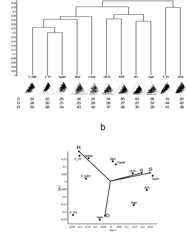
3.3 Community structure in Central European mixed forests.
401
The species composition of eleven organism groups (herbs, saplings, understorey bryophytes, 402
epiphytic bryophytes, epiphytic lichens, terricolous saprotrophic fungi, wood-inhabiting 403
fungi, ectomycorrhizal fungi, spiders, carabid beetles, and birds1) was surveyed in mixed 404
temperate forests in West-Hungary (North 46°51’-55’, East 16°07’-23’, for map see Fig.
405
S2.4).
406
In this case study, sampling was designed in a way that all organism groups were surveyed in 407
all the 35 sample sites (see Appendix S2, for details). As a consequence, the comparison of 408
point scatters within the ternary plots simplifies to the direct measurement of shift (Eq. 7).
409
The matrix of resulting Manhattan distances was then subjected to UPGMA clustering and 410
PCoA, as in the above two case studies.
411
1 The latter three are monophyletic taxa, the first two are largely independent of taxonomy, the others represent
a
412
Dissimilarity
0.34 0.32 0.3 0.28 0.26 0.24 0.22 0.2 0.18 0.16 0.14 0.12 0.1 0.08 0.06 0.04 0.02
0 F_MYC F_W Spider Bird Carab LICH B-EP B-S Sapl F_TS Herb
S 22 22 25 34 34 34 45 43 38 15 20 D 28 20 21 23 26 29 27 27 33 44 42 R 50 58 54 43 40 37 28 30 29 41 38
413
b
414
Axis 10 0.05 0.1 0.15 0.2 0.25 -0.05
-0.1 -0.15 -0.2 -0.25
Axis 2
0.15 0.1 0.05 0 -0.05 -0.1 -0.15 -0.2 -0.25
F_TS F_W
F_MYC Spider
Herb Bird
Carab LICH
Sapl B-S
B-EP
S R
D
q
415
Fig. 6. (a) UPGMA dendrogram for the forest community example. The SDR-simplex 416
diagrams are shown in miniature under each label together with the percentage contributions 417
from the S (right corner), D (left corner) and R (top corner) fractions, (b) PCoA ordination for 418
axes 1-2; scaling of arrows: 0.25 = unit correlation. Abbreviations as in Table 1.
419
420
The dendrogram (Fig. 6a) separates organism groups in which species replacement (R) is the 421
dominant component (on the left: ectomycorrhizal fungi, wood inhabiting fungi, spiders, 422
birds, carabids), from similarity (S) dominated groups (in the middle: epiphytic bryophytes, 423
understory bryophytes and saplings), and beta diversity dominated groups for which the D 424
and R components had similarly high importance (on the right: terricolous saprothrophic 425
fungi, herbs). Epiphytic lichens had an intermediate position between the R and S groups. The 426
ordination (Fig. 6b) agrees well with the agglomerative classification in revealing meta- 427
structure of the organism group data. PCoA axis 1 (20%) represents a gradient from high 428
levels of species replacement (R component, negative side) to relatively high similarity (S, 429
positive side) as expressed by its high correlation with R (r1R = –0.83) and S (r1S = 0.96).
430
Matrix fill has high correlations with similarity (rqS = 0.89) and axis 1 (r1q = 0.82). Ordination 431
axis 2 (15%) is the most correlated with richness difference (r2D = –0.94).
432
The overall picture on point clouds within the SDR triangles is that different organism groups 433
develop greatly different community pattern in the same sites. The points in many cases form 434
a narrow triangular shape with the tip near the D vertex and the base on the right, richness 435
agreement (R-S) edge. Most of the organism groups with high beta diversity have a relatively 436
high species richness (fungi groups, herbs, birds) and low level of matrix fill (fungi groups, 437
herbs, spiders, Table 1). It means that in these organism groups (especially for fungi) the 438
proportion of rare species (occurring only in one or two plots) is very high.
439
This study indicates that in some organism groups high beta diversity, while for others higher 440
similarity is the dominant structural component. The high beta diversity and low nestedness of 441
fungus assemblages compared to other sessile organism groups have been proved for 442
saproxylic communities (Halme et al. 2013; Heilmann-Clausen et al. 2014). This high beta 443
diversity of the fungal groups could be related to the methodology of sampling which focused 444
on sporocarp inventory. Similarly to this study, the species replacement component of beta 445
diversity for breeding bird assemblages had higher importance than richness difference (low 446
level of nestedness effect, Si et al. 2015). In vascular plant and beetle assemblages of 447
European beech forests, species replacement had much stronger effect on beta diversity than 448
nestedness (Gossner et al. 2013), while for epixylic and epiphytic bryophytes in this 449
community nestedness had higher importance (Táborska et al. 2017). For forest bryophytes 450
and lichens, especially for epiphytic and epixylic assemblages, a high degree of nestedness is 451
detected in many forest types (Hylander & Dynesius 2006; Nascimbene et al. 2010). Spider 452
and carabid beetle communities of this study had similar metacommunity structure with 453
relatively even S-D-R distribution. For spiders, the dominance of species replacement and low 454
level nestedness has been shown (Carvalho & Cardoso 2014).
455
The similar environmental drivers only partly support groups based on the simplex structure.
456
Within the beta diversity dominated clusters, the species composition of the three fungus 457
groups and spiders is determined mainly by tree species composition, and forest microclimate 458
(Samu et al. 2014, Kutszegi et al. 2015). However, herbs also exhibiting high beta diversity 459
are influenced mainly by other variables (e.g., light conditions, tree species diversity and 460
shrub layer density, Márialigeti et al. 2009, 2016; Tinya et al. 2009). Epiphytic bryophytes 461
and lichens also share some common environmental drivers such as shrub density and humid 462
microclimate (Király et al. 2013; Ódor et al. 2013). Birds are related to different drivers than 463
the other organism groups like tree size, dead wood amount and understory cover (Mag &
464
Ódor 2015).
465 466
3.4 Community recovery of arthropods in Florida: Rey’s defaunation experiment.
467
In order to test the equilibrium theory of insular biogeography, Rey (1981) investigated the 468
arthropod fauna of six islets in northern Florida. These islets are from 56 m2 to 1023 m2 in 469
area, and are located at a distance of 29 m to 1752 m from the mainland. The vegetation of the 470
study area was a monodominant stand of smooth cordgrass (Spartina alternifolia Loisel.). At 471
the beginning of the experiment, the terrestrial arthropods of the islets were killed by 472
insecticides. The arthropod fauna was then recorded in weekly intervals for a year to monitor 473
the recolonization process. Details are given in the original publication by Rey (1981). We 474
took the species by islands data from 20 points of time (weeks 9-26, 31 and, finally, 53), 475
made available as a supplement to the nestedness calculator program package developed by 476
Atmar & Patterson (1995).
477
478
Axis 1
0.2 0.15
0.1 0.05
0 -0.05
-0.1
Axis 2
0.12 0.1 0.08 0.06 0.04 0.02 0 -0.02 -0.04 -0.06 -0.08 -0.1 -0.12
31 26
20 22 19
21
23 25
24 18
17
15
13
12
10 11
9 16
53
S
D
R q
14
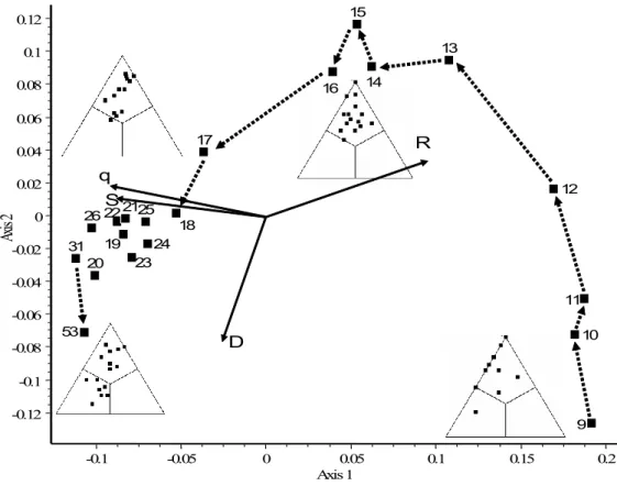
479
Fig. 7. Principal coordinates ordination of 20 data matrices from the island recolonization 480
experiment in northern Florida. Simplex plots are shown for weeks 9, 14, 25 and 53. Note the 481
S (right corner), D (left corner) and R (top corner) fractions in each plot. Dotted arrows 482
connect subsequent weeks, but those are omitted for weeks 18 to 31 for clarity. Scaling of 483
solid arrows: 0.1 = unit correlation. See Table 2, for centroids and matrix fill percentages.
484 485
This survey provided data suitable for demonstrating the performance of our procedure in the 486
analysis of pattern development for the same set of localities (i.e., islets) over time. We 487
therefore used Eq. 7, the direct method to express pattern dissimilarity between points of time.
488
We feel that hierarchical classification is less relevant to this situation, and suggest that the 489
problem of monitoring temporal changes is sufficiently approached by PCoA. The results are 490
shown in Fig. 7 for the first 2 ordination axes (accounting for 54% and 16% of variance, 491
respectively). Four simplex plots, from weeks 9, 14, 25 and 53, are superimposed to the 492
ordination near the points they represent.
493
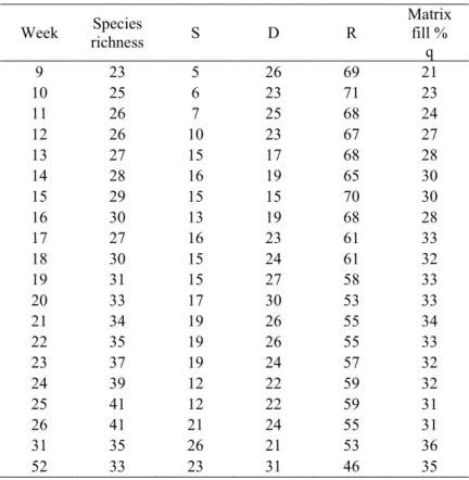
Table 2. Main data properties and SDR centroids for data from Rey’s island recolonization 494
experiment.
495
Week Species
richness S D R
Matrix fill %
q
9 23 5 26 69 21
10 25 6 23 71 23
11 26 7 25 68 24
12 26 10 23 67 27
13 27 15 17 68 28
14 28 16 19 65 30
15 29 15 15 70 30
16 30 13 19 68 28
17 27 16 23 61 33
18 30 15 24 61 32
19 31 15 27 58 33
20 33 17 30 53 33
21 34 19 26 55 34
22 35 19 26 55 33
23 37 19 24 57 32
24 39 12 22 59 32
25 41 12 22 59 31
26 41 21 24 55 31
31 35 26 21 53 36
52 33 23 31 46 35
496
The arrangement of simplex diagrams in the ordination follows an obvious horseshoe pattern, 497
otherwise very typical for community data with a single dominant environmental gradient to 498
which all species respond in a unimodal fashion (Podani & Miklós 2002). Thus, the presence 499
of the horseshoe in the present case appears to indicate a one-directional temporal trend 500
regarding changes of community pattern on the islands. In this, with the exception of week 501
15, we cannot see seasonal variations and strong fluctuations that were otherwise observed for 502
various diversity statistics by Rey. As also shown by Podani & Schmera (2011), there is a 503
fairly monotonous increase of matrix fill, S and nestedness over time; therefore, replacement 504
and beta diversity exhibit the opposite behaviour while changes of richness difference appear 505
less consistent (Table 2). This is expressed quite well with the product moment correlation 506
coefficients calculated between axis 1 and S, R and q (r1S = –.81, r1R = .88, r1q = –.92) of 507
which the correlation with matrix fill is the highest. However, the second axis may also be 508
interpreted in terms of the SDR values, namely the correlation with richness difference is r2D
509
= –.76, showing some less obvious trend that richness difference first decreases and then 510
increases over time. This suggests that in this case study the horseshoe pattern is not a 511
mathematical consequence of a long, unidimensional background gradient, but the 512
manifestation of two, largely independent changes of community pattern.
513
As Rey (1981) reported, the first species appeared c. 4-5 weeks after treatment and then the 514
total number of species started to increase rapidly. Re-occurrence of species on particular 515
islets was accidental, however. Therefore, this pioneer stage is characterized by very high beta 516
diversity as is indicated by many points lying on the left side of the SDR plot: the 517
corresponding pairs of islands had no single species in common (week 9). Then, extinctions 518
and immigrations dominated until week 18 with further increases in species number. This 519
second period is shown by the increased concentration of points inside the upper third of the 520
triangle (the species replacement sector). As Rey observed, species richness reached the 521
original levels in approximately 20 weeks and oscillated around these values until the end of 522
the experiment. Our analysis reveals that not only species richness but community pattern was 523
also oscillating in this period, as shown by little changes in the ordination. The simplex plot 524
for the last week (53) shows recovery to the original state: richness difference has increased as 525
expected, and half of the points moved into the richness difference sector of the triangle. It is 526
the manifestation of the classical species/area relationship. That is, by the end of the 527
experiment the normal conditions are observed again because the islets differ considerably in 528
size so that they maintain different levels of alpha diversity.
529 530
4. Discussion 531
Methods of multivariate analysis have been commonly used in ecology and biogeography to 532
reveal non-random structure implied in presence-absence data matrices. Comparison of their 533
results is a common practice whenever interest lies in evaluating the relative importance of 534
user decisions made during sampling and data processing, in quantifying the effect of 535
choosing between descriptor variables, and in the discovery of underlying factors affecting 536
these results (Podani 1989, Lengyel & Podani 2014 and references therein). Generally, such 537
studies are performed on (dis)similarity matrices (e.g., matrix correlation, Mantel 1967, 538
Sneath & Sokal 1973, Hubert 1983), dendrograms (Rohlf 1974), partitions (Arabie &
539
Boorman 1973), and ordinations (Gower 1971, 1975); but see Podani (2000, Chapter 9) for a 540
more complete account of the issue. Application of these types of results in comparisons 541
always implies some loss of information. Calculating dissimilarities from raw data usually 542
ignores the relationships between variables by reducing the comparison to a single number.
543