L. REVICZKY - J. HETHÉSSY

MAGYAR TUDOMÁNYOS AKADÉMIA

SZÁMÍTÁSTECHNIKAI ÉS AUTOMATIZÁLÁSI KUTATÓ INTÉZETE

A G E N E R A L A P P R O A C H FOR D E T E R M I N I S T I C A D A P T I V E R E G U L A T O R S B A S E D ON E X P L I C I T I D E N T I F I C A T I O N

L . REVICZKY - J. HETHÉSSY

T a n u l m á n y o k 1 4 9 / 1 9 8 3

Főosztályvezető:

REVICZKY LÁSZLÓ

ISBN 963 311 163 3 ISSN 0324-2951

A TANULMÁNYSOROZATBAN 1 9 8 2 ’ BEN MEGJELENTEK

130/1982 Barabás Miklós - Tőkés Szabolcs: A lézer printer képalkotás hibái és optikai korrekciójuk

131/1982 R G - 11/KNYVT "Szisztemü upravlenija bazani dannüh i informacionnüe szisztemü" Szbornik naucsno-iszszle- dovatel'szkih rabot rabocsej gruppü RG-II K N W T , Bp. 1979. T o m I.

132/1982 RG-II / K N W T T o m II.

133/1982 RG-II K N W T T o m III.

134/1982 Knuth Előd - Rónyai Lajos: Az SDLA/SET adatbázis lekérdező nyelv alapjai /orosz nyelven/

135/1982 Néhány feladat a tervezés-automatizálás területéről Örmény-magyar közös cikkgyűjtemény

136/1982 Somló J á n o s : Forgácsoló megmunkálások folyamatainak optimálási és irányítási problémái

137/1982 KGST 1-15.1. Szakbizottság 1979. és 80. évi előadásai

138/1982 Kovács László: Számitógép-hálózati protokollok formális specifikálása és verifikálása

139/ 1982 Operációs rendszerek elmélete 7. visegrádi téli iskola

- 5 ^-

1.INTRODUCTION

The automatic adjustment of regulators for industrial processes has received particular

attention for many years. Apart from the complexity of the regulator, there are indeed practical

situations requiring automatic tuning or adaptivity in order to ensure better control performance:

- the parameters of the system to be controlled vary from time to time

- the system itself is actually nonlinear and the parameters of the linearized process model depend on the operating points

- an automatic adjustment of the regulator parameters is required, because of the complexity or slow dynamics of the process.

The present state of the research works in the field of the adaptive control reflect a synthesis of the classical principles and the results of the seventies, when the idea of self-tuning control got so attractive and popular.

The subject of this work is the adaptive servo- regulatory problem. Aiming the practical applica­

bility pole/zero assignment regulators will be con­

sidered rather than optimal strategies. The noise rejection will be designed for deterministic, step­

wise disturbances, however to show the generality of the presented design base, the stochastic noise rejection problem will be shortly discussed,as well.

Since the early paper of Peterka [38] and Äström and Wittenmark [5] the self-tuning regulators mean a very attractive class of adaptive controllers.The basic self-tuning control algorithms were developed for the rejection of stochastic disturbances acting on the process to be controlled. There was some early try to extend the self-tuning regulators to include constant set point, too [25]. Aiming the practical applicability of the self-tuning regula­

tors the basic self-tuning idea was extended by Clarke and Gawthrop [ 14,15,16].Their generalized self-tuning controller minimizes a loss function incorporating terms relating to the servo and regu­

latory performance, thus it can be interpreted as a model-referenee strategy, as well [ 221 .

- 7 -

A different suboptimal approach was given by Wellstead et al. [47,49]. This method detunes the optimal, minimum variance controller by prescribing poles and zeros for the closed loop system. The servo problem was also solved | 48], but in a rather complex w a y .

A general and systematic approach was given by Äström et al. [ 7,8] for the deterministic servo p r o b ­

lem. In addition to the general pole/zero placement design structures a classification for the adptive schemes was also suggested [ 7], namely the explicit and implicit schemes were introduced. Unlike the im­

plicit schemes the explicit schemes require the iden­

tification of the plant, thus the explicit and im­

plicit schemes are often referred as indirect or direct schemes, respectively[36].

It is well known [6,7,33,40,42,43,44] that the cancellation controllers which are to cancel poorly damped zeros or zeros of inverse unstable processes result in rippling intersampling behaviour and exhibit the infinite sensitivity problem, respectively. To avoid these difficulties a number of design strategies have been developed so far, which can be essentially classified as cancellation methods and methods m i n i ­ mizing a general loss function. The cancellation con-

trollers allow the process zeros outside a given de­

sign region to appear in the closed loop system, while the general loss functions incorporate terms relating to the control effort, but in this latter case the loss function adjustment is far not a trivial design step [2,3].

The relationships between the mentioned design methods and some links with the frequency domain considerations were discovered in a very interesting way by Allidina and Hughes [ 1,2,3,27]. A new pole placement design method suitable for the adaptive control of nonminimum phase systems was presented by Berger[ll], where the pole place­

ment was also achieved by the choice of an appropriate loss function, but the suggested method requires a matrix inversion in every step.

Regarding to the cancellation controllers the adaptive control can be based on both implicit and explicit schemes.

As far as the implicit or direct methods are concerned, the fundamental difficulty is caused by the fact, that the parametrization leads to an estimation problem bili­

near in parameters. The solution given by Áström needs further analysis, while another approach presented by

Hetthéssy et al.[24j suffers from the numerical difficulty of finding the common roots of two updated regulator po-

- 9 -

lynomials. A direct adaptive control strategy for c o n ­ tinuous nonminimum phase systems has been developed r e ­ cently by Elliott [l8]. All these direct methods estimate an extended parameter vector. A quasi-direct method by Lozano and Landau ( 36] updates the process and regulator parameters in each step and the estimated process p a r a ­ meters are used to filter the input/output observations.

The explicite schemes are usually based on a Diophantine equation to be solved. In addition to this, in general case the estimated process numerator has to be factorized to separate the process zeros to be and not to be cancelled [7,8]. If no process zeros are to be cancelled the fa c t o ­ rization is not required. For this latter case Goodwin [23]] gave a detailed analysis including a local conver­

gence proof. Similar results were presented by Boland and Giblin [ 12] using appropriate saturation for the control a c t i o n .

However, an early attempt is known to compute the regu­

lator parameters in a very simple way, without solving any identity [30]] . A number of works [ 19,26,29,35,51 ] have re­

called this explicit method recently, but only stable p r o ­ cesses have been considered so far.

In this work the deterministic servo-regulatory problem is considered and solved, treating well known results and giving some innovations. Two basic control structures are established in different forms to control both stable and unstable, as well as minimum and nonminimum phase processes.

The first structure requires moderate computations, and the known results are extended for integrating and unstable systems, while the second structure creates a predictive form based on a polynomial equation to be solved. In both structures prespecified zeros and poles can be placed into the closed loop system, regarding to follow a reference model and the noise rejection, as well. The influence of the prespecified zeros and poles on the control action is shown. For the adaptive solution the explicite scheme is proposed, however the implicit adaptive solutions are also overviewed and a new derivation of the direct adaptive algorithm by Äström is also presented.

As an important motive from practical point of view, saturations in the control input are also taken into con­

sideration. The theoretical results are illustrated by hybrid simulations.

11

2. DETERMINISTIC SERVO REGULATOR DESIGN FOR PROCESSES WITH KNOWN PARAMETERS

Consider the single input single output, discrete time linear systems given by

y (t) + a^ y (t - 1) + ...+any (t-n)=bQu (t-d) + + b „ u (t - d - 1 )+ ...+b u(t-d-m)

1 m

where t=0,1,2,... denotes the discrete time instants, u and y stand for the system input and output, respectively. The discrete time delay d is assumed to be d>0.

Using the backward shift operator z -1 and introducing the polynomials

■“ n A (z ) = 1 + a 1z + . . . + anz

and

. -1. , -1 , -m

B (z ) = b + b.z + . . . + b z

o 1 m

the discrete transfer function of the process is obtained by

y(t) = z d u(t) , (2-1) A (z” )

- 1 -1

where A(z ) and B(z ) are relatively prime polynomials (they have no common r o o t s ) .

The aim of the control is to ensure a closed loop system to follow the output of a reference model

-1 - 1

N(z )/M(z ) as close as possible. A general control structure involving a precompensator , a serial regulator W 2 and a feedback compensator is shown in Figure 2-1. For the sake of simplicity the argument z -1 will be dropped in the sequel. As the reference model driven by a reference signal y (t) is placed

into the feedforward path, the optimal overall transfer function between the reference model and the process output is z d , which gives

w , w 2

1

1+W W 7 z d 2 3 a

z-d

or equivalently

W 2B (W.J-W z A (2-2)

- 13 ^-

F i g u r e 2 - 1.

Fi gur e 2- 2 .

F i g u r e 2 - 3 .

Eq. (2-2) shows that an infinite set of {W^, / W^}

exists to meet the optimality, however, they ensure different noise rejection, as does not appear in the closed loop. Assuming deterministic, step-wise

disturbances acting on the process output, the complete noise rejection takes d steps in the optimal case.

Designing also the dynamics of the noise rejection we have

1

1+ W 2W 3 ! Z'd

(2-3)

where the polynominals

V V 1 Z

- 1 -n

v z v nv

and

T t +

o

V

(2-4)

contain prespecified zeros and poles in the noise rejection by Eq.(2-3). Now Eq.(2-2) and E q . (2-3) lead to

15 -

thus choosing w 3 V

W = T 1

(2-5)

(2-6)

and

w 3 = v ,

a serial regulator

(2-7)

A B (T-Vz )

is obtained (Figure 2-2).

Eq.(2-3) shows that to avoid the steady-state errors of the noise rejection

V(1 ) = T(1 ) (2-9)

m u s t hold, a s

= 0.

z = 1 (2-1 0)

It is remarkable that the condition by Eq. (2-9) causes the serial regulator to be of integrating

type, namely the denominator B(T-Vz ^) has a root of z1 = 1 , as T (1) - V (1).1 = 0.

The c l o s e d loo p p r o p e r t i e s c a n b e s u m m a r i z e d as f o l l o w s :

Poles Zeros

y_ -> y M N

e -*■ y T V

Overall transfer function N

M

It is seen that all the closed loop zeros and poles can be prespecified by using appropriate design polynomials M,N,T and V.

Results for the special choice of N=V and M=T,

- 17 -

as well as for N=V=M=T=1 are shown in Figure 2-3 and 2-4 , respectively.

Based on Figure 2-2 the characteristic equation is

1 +

B (T-Vz d )

B -d - z = 0

or equivalently

ABT = 0 (2-11)

which shows that because of the infinite sensitivity problem [7,14,33,34,43] the previously proposed

algorithm is applicable only for stable, minimum phase systems. To make the citation easier the strategy shown in Figure 2-2 will be referred as optimal 3 structure, or simply as ßQ structure in the sequel. To summarize its applicability it should be underlined that it is inadmissably sensitive when controlling unstable or nonminimum phase systems. On the other hand, in the knowledge of the process parameters, the regulator parameters can be directly computed by

F i g u r e 2 - 4 .

F i g u r e 2- 5.

F i g u r e 2-6.

19 -

W1 T

W A

2 B(T-Vz-d ⁽2-1 2)

W3 V

to ensure the prespecified closed loop zeros and po l e s .

In the sequel it will be shown that the poles of the process do not appear necessarily in the serial regulator. Define polynominals F and G by

then applying Eq. (2-13) - similarly to the multivariable case [32] - for the process output

T = AF + VGz-d

(2-13) t

Ty(t+d) = (AF+VGz d ) y (t+d)

= AFy(t+d)+VGy(t)=BFu(t)+VGy(t), (2-14)

is obtained as an errorless prediction form for Ty(t+d). The polynominals introduced by Eq.(2-13) are unique using F and G with degrees

F = fn + f 1Z o 1 + •**+ f n +d-11Z °v v

g = g 0 +g-,z 1 + •••+ gn-iz~ (n_1)

(2-15)

As the optimality has been defined by

y (t+d) = | y r (t) , (2-16)

E q s . (2-14) and (2-16) give

f T y (t) - VGy(t)

u (t ) = — ----- --- (2-17) B F

for the control input (Figure 2-5). The condition defined by Eq. (2-16) can be considered as a trivial design step, as well.

T h e o v e r a l l t r a n s f e r f u n c t i o n r e l a t i n g to the o u t p u t n o i s e is d e t e r m i n e d b y

1 AF

. ^ VG B -d 1 + — . — z

BF A

VG -d

— z , (2-18) T

which shows that in addition to the design polynomials the noise rejection depends on G, too. For example in

- 21

case of V=T=1 and G(1)=1 the complete noise rejection takes (nG+d) steps.

The presented algorithm will be referred

optimal a, or aQ strategy in the sequel. Summing up its main properties it is seen from its

characteristic equation

BT = 0 (2-19)

that it can be applied for minimum phase systems and the regulator parameters are to be computed by solving a polynomial equation (Eezout identity).

It has been shown so for that the a and ß

o o

strategies are equally unable to control nonminimum phase systems. To clear up the importance of this problem it has to be emphasized that unlike continuous systems, nonminimum phase discrete systems do not mean a narrow class at all, as sampled minimum phase

continuous systems exhibit nonminimum phase properties rather frequently [7,8,33,34,41,49],

To control nonminimum phase discrete or sampled continuous systems suboptimality in the design

procedure will be introduced in the sense of allowing the unstable or poorly damped zeros to appear as

zeros of the closed loop system [40].

Factorize the numerator of the process by

B = B 1 • B 2 (2-20)

with B2 (1)=1f where B 2 contains the zeros not to be cancelled [7,8] :

B 1 = B (z 1 ) = b 1 A + b 1 1 z 1+ . . . + b. z m l

• I 1u II \fm ^

B 2 = B 2 (Z_1 = b 2 0+b 21Z ' 1 + - - - + b 2, m 2'” 2

m^ + m 2 = m

(2-2 1)

b 20 + b 21 +> *,+ b 2 , m 2 1 ’

To ensure an overall transfer function of B 2z between the reference model and the process output we have

r7 TT A -d W 1W 2 B Z 1 + W-W, I z"d

2 3 A

- 23 -

o r e q u i v a l e n t l y

H 2B 1 ,W1 - B 2W 3

z -d.) = (2-22)

S i m i l a r l y , B 2 is a l l o w e d to a p p e a r in t h e n o i s e r e j e c t i o n in t h e f o l l o w i n g way:

1

1

w w

2 3

B - d

z

(2-23)

wheref rom

T V

is o b t a i n e d a g a i n . B y c h o o s i n g

(2-24)

W 1 = T (2-25)

a n d

w 3 = v

the serial regulator given by Eq. (2-22) is

A W =

2

B 1 (T-B2V^z d )

(2-27)

The presented suboptimal ß strategy (8^) is shown in Figure 2-6. Results with N=V and M=T, as well as with N =V=M=T=1 are shown in Figure 2-7 and 2-8 ,

respectively.

The characteristic equation for the general case is

A B 1T = 0 (2-28)

while the closed loop properties can be summarized as follows:

y r+ y

e -> y

Poles M

T

Z e r o s

N. B.

V. B.

Overall transfer function NB.2 -d

z M

- V B 2 -d 1 - --- z

(2-29)

prespecified derived

By Eq. (2-28) it can be stated that the ßg strategy can be applied for any stable process, and the

regulator parameters can directly be computed having the process numerator appropriately factorized.

- 25 ^-

Figure 2-7.

/

F i g u r e 2 - 8 .

F i g u r e 2 - 9 .

The control input now can be expressed by

N

[ - T yr (t) - Vy(t)] A u<t) = ---

B 1 (T - V B 2z_ d )

A rN , ,, , V .. ,.

B 1 M Y r (t)~ TS

(2-30)

which clearly shows the direct influence of the design polynomials on the control action.

It is remarkable that if no process zeros are to be cancelled the factorization B=B^B2 is not required, as in this case

B 2 = — -— (2-31 )

B (1 )

and

B 1 = B (1 ) (2-32)

This special, practical minded choice is discussed by several authors [19,29,35,51 ].

Introducing further speciality by N=V and T=1 W 2W 2 becomes

w 2w 3 AV_____

- V B z _d B (1 )

(2-33)

- 27

This result was introduced by Kalman [30] with V = 1 , treated by Favier and Guillermin [19] , used by Kurz et a l . [35] with V=1 as DB1 and with

V=v +v„z _ 1 as DB2 dead-beat regulator, as well as o 1

applied by Zimmermann [51] with a general, parameter optimizable plynomial V.

To illustrate the practical possibilities offered by the design polynomials and to show that the general approach includes well-known algorithms [29, 35 ] as special cases, consider a design with

M = T = 1

N = V = v + v . z o 1 v o + V 1 = 1

y (t) = Y , if t ä 0 and

J r o

y (t) = 0 otherwise,

B 2 = B B (1 ) B 1 = B ( 1 )

Using Eq. (2-30) with e(t)=0 we have

u(t) = — -— (v + v.z 1) y (t) , B (1 ) °

(2-34)

which gives

v Y u (0 ) = -- (2-35)

B (1 )

u(1)

a.v Y 1 o B (1 )

o v Y o o B (1 )

+ V 1Y

B (1 Y

= a u(0) + -- — . (2-36) B (1 )

It is seen that the first value of the control input can be influenced by v , however choosing too small a u(0), a large u(1) could be required. A reasonable choice for v is obtained if

o

u(1) < u (0) (2-37)

is ensured. Combining Eqs. (2-36) and (2-37)

S v < 1 o 1 -a.

gives a practical region for v

(2-38)

- 29 -

In the s e q u e l a p r e d i c t i v e s u b o p t i m a l s t r a t e g y (ag ) w i l l be d e r i v e d . D e f i n e F a n d G b y

T A F + B 2G Vz-d

(2-39)

w i t h

F =

W

v 2

- (n + m n +d-1 )

z v 2

(2-40)

a n d

G = g o +g-,z 1 +...+ g n-1 z *n - 1 * , (2-41)

U s i n g Eq. (2-39) w e h a v e

_ o

T y (t+d) = (AF + B 2G Vz )y(t+d) =

= A F y(t+d)+B2G V y(t) = B F u (t )+ B2G V y (t )=

= B 2 [B 1F u (t ) + G V y (t)] . (2-42)

C o m b i n i n g Eq. (2-42) and

y (t+d)

M B 2y r (t) (2-43)

as a c o n d i t i o n of t h e s u b o p t i m a l i t y the c o n t r o l input is g i v e n b y

^ . T y r (t) - GVy(t)

u ( t ) = --- , (2-44)

a n d the c l o s e d loo p s y s t e m is s h o w n in F i g u r e 2-9.

T h e n o i s e r e j e c t i o n of t h e a s t r u c t u r e is s

1

1 + ^BGVz

A B 1 F

B 2GVz

--- , (2-45)

T

a n d thus

T (1 ) = G (1 ) V (1 ) (2-46)

w i l l e n s u r e t h e e l i m i n a t i o n of s t e a d y - s t a t e e r r o r s , as B 2 (1)=1. T a king Eq. (2-46) i n t o c o n s i d e r a t i o n Eq. (2-39) g i v e s

A {1 ) F (1 ) = 0 (2-47)

again. F o r p r o c e s s e s w i t h no i n t e g r a t o r ( s ) F = F ' ( 1 - z ^) s h o u l d be u s e d to s a t i s f y t h e a b o v e r e q u i r e m e n t . The c l o s e d l o o p p r o p e r t i e s e n s u r e d b y t h e a g s t r a t e g y

31

can be s u m m a r i z e d as follows:

P o l e s Z e ros

-* y

e -> y

M N

. B,

v .

2

O v e r a l l t r a n s f e r f u n c t i o n N B 2z-d

M

1 ^-

(2-48) B 2GVz-d

T p r e s p e c i f i e d d e r i v e d

T h e c h a r a c t e r i s t i c e q u a t i o n is

B 1T = 0 (2-49)

w h e r e f r o m it is seen th a t t h e a s t r u c t u r e can b e s

u s e d to c o n t r o l a n y k i n d of p r o c e s s e s .

It is r e m a r k a b l e that a s s u m i n g s t o c h a s t i c o u t p u t d i s t u r b a n c e s d r i v e n b y w h i t e n o i s e t h r o u g h a n o i s e m o d e l of C / A [4], t h e c l o s e d l o o p t r a n s f e r f u n c t i o n

is

C A

(1 B 2 GV T

C ( T - B 2G V z _ d ) A T

C A F _ CF

A T T

(2-50)

w h e r e f r o m a c h o i c e b y

T T ' C (2-51)

g i v e s the d e t u n e d s u b o p t i m a l c o n t r o l i n t r o d u c e d b y W e l l s t e a d e t . al [47, 49] . S e e a l s o in C l a r k e [17].

N o t e t h a t the c h o i c e of = 1 r e p r o d u c e s the o p t i m a l s o l u t i o n , i.e. a l l t h e p r o c e s s z e r o s a r e to be c a n c e l l e d , w h i l e s p e c i f y i n g = B/B(1) c o r r e s p o n d s to a d e s i g n p r i n c i p l e of n o p r o c e s s z e r o c a n c e l l a t i o n . T h i s l a t t e r c a s e c o u l d b e v e r y advantageous f r o m p r a c t i c a l p o i n t of v i e w , n a m e l y t h e f a c t o r i z a t i o n B = B ^ B² d o e s n o t n e e d to s o l v e t h e e q u a t i o n of zm B=0.

To i m p r o v e the s t r u c t u r e f o r t h e c o n t r o l of u n s t a b l e p r o c e s s e s d e f i n e t h e s e r i a l r e g u l a t o r b y

A1

W2 (2-52)

B„ F1

w h e r e

(2-53)

a n d A 2 c o n t a i n s all t h e u n s t a b l e p o l e s a n d it is n o r m a l i z e d b y A 2 (1)=1. U s i n g Eq. (2-22)

(2-54)

- 33 -

is o b t a i n e d , and c h o o s i n g W ^ = T a n d W^=GV a p o l y n o m i a l e q u a t i o n

T = A 2F (1-z‘ V + B 2 GV z_ d (2-55)

d e t e r m i n e s the r e g u l a t o r p o l y n o m i a l s F a n d G.

F r o m t h e c o n d i t i o n of s t e a d y - s t a t e e r r o r s f o r k = 0

F = F ' (1- z _ 1 )

h a s to b e s u p p o s e d a gain, w h i l e f o r k > 0 t h e c o n d i t i o n by

A (1 ) F (1 ) = 0

is a u t o m a t i c a l l y f u l f i l l e d .

T h i s s o l u t i o n e x h i b i t s t h e p r o p e r t i e s of bo t h the a a n d ß s t r u c t u r e s , thus it w i l l be r e f e r r e d as a Y s t r u c t u r e ( F i g u r e 2-10).

s

«

A s a sp e c i a l c a s e c o n s i d e r s t a b l e s y s t e m s (A2 =1) w i t h o n e i n t e g r a t o r (k = 1). F r o m Eq. (2-55) G = g Q is o b t a i n e d and

T = F (1 - z ” 1 ) + g QB 2V z ( 2 - 5 6 )

F i g u r e 2- 10.

F i g u r e 2- 11.

- 35 -

Substituting z=1 into the above equation we have

t (1) = g Q v (1) (2-57)

T h i s i m p l i e s t h a t z the p o l y n o m i a l F can

_ ^ T, — d T - g B~Vz

„ ^o 2

-1 be

V f

_

is a r o o t of T-g B„Vz a n d

^o 2 c o m p u t e d e x p l i c i t e l y by

. + f

n +m„+d-1 v 2

+m2+ d - 1)

(2-58)

S u m m i n g u p the a p p l i c a b i l i t y of the y s s t r u c t u r e , t h e c h a r a c t e r i s t i c e q u a t i o n b y

A ^ T = 0 (2-59)

shows that it can be applied for all kind of processes.

Note that the order of the polynomial equation (2-55) to be solved is lower by the number of the stable poles than in case of the ag strategy.

In a d d i t i o n to thi s it g i v e s a n e x p l i c i t e x p r e s s i o n f o r the r e g u l a t o r p o l y n o m i a l s in c a s e of s t a b l e p r o c e s s e s w i t h o n e i n t e g r a t o r .

A l l t h e p r e s e n t e d s t r u c t u r e s a r e r e v i e w e d in T a b l e

- 37 -

2-1. N o t e th a t t h e p o l y n o m i a l e q u a t i o n s l e a d to a set of l i n e a r e q u a t i o n s , h o w e v e r the r e s o l u t i o n c o u l d be v e r y s e n s i t i v e [9, 17].

2.1. D e s i g n c o n s i d e r a t i o n s for t h e c a n c e l l a t i o n of t h e p r o c e s s z e r o s

In this c h a p t e r the d e s i g n r e g i o n s f o r the

p r o c e s s z e r o s to b e c a n c e l l e d wi l l b e c o n s i d e r e d . As t h e p r o c e s s z e r o s to be c a n c e l l e d m e a n p o l e s for t h e r e g u l a t o r , t h e d y n a m i c b e h a v i o u r of t h e c o n t r o l i n p u t d e p e n d s on t h e c a n c e l l e d zeros. It is w e l l - - k n o w n that a n y r e g u l a t o r p o l e o u t s i e d t h e u n i t c i r l e c a u s e s an e x p o n e n t i a l l y g r o w i n g c o n t r o l input.

H o w e v e r , r e g u l a t o r poles w i t h i n the u n i t c i r c l e c a n a l s o c a u s e r i p p l e s in the c o n t i n u o u s p r o c e s s o u t p u t

[34, 40, 43, 44 ], if the o s c i l l a t i o n of the control i n p u t is n o t d a m p e d a p p r o p r i a t e l y . To a v o i d t h e d i s a d v a n t a g e o u s i n t e r s a m p l i n g b e h a v i o u r of t h e c o n t i n u o u s p r o c e s s o u t p u t t h e d i s c r e t e p r o c e s s z e r o s to b e c a n c e l l e d h a v e to l i e i n s i d e a d e s i g n r e g i o n .

F o r c o n t i n u o u s time s y s t e m s the a n g l e b e t w e e n t h e n e g a t i v e rea l axis a n d t h e li n e f r o m the o r i g i n to the d o m i n a n t p o l e s d e t e r m i n e s t h e damp i n g .

S i m i l a r c r i t e r i a e x i s t for s a m p l e d d a t a syst e m s . To s h o w t h e c r i t i c a l c urves of c o n s t a n t d a m p i n g c o n s i d e r a c o n t i n u o u s s y s t e m of a d o m i n a n t pol e pai r

1

1 + 2 Ts + T2 2 s

(2-60)

w h i c h h a s a step r e s p o n s e e q u i v a l e n t d i s c r e t e for m by

b + b. z

o 1

1 + z^{- 1} - 2 + a 2Z

(2-61 )

w h e r e

a1 - 2 e C O S X (2-62)

a2 = e-2£x (2-63)

a n d x s t a n d s f o r t h e r e l a t i v e s a m p l i n g [33] :

x h

T

N o w the p o l e s of the s a m p l e d s y s t e m a r e g i v e n by t h e r o o t s of

2 2

z A = z + a^z + a^ 0. (2-64)

T h e r o ots of Eq. (2-64) a r e

z1,2 ^{e V}

(2-65)

a n d the c r i t i c a l c u r v e s f o r so m e g i v e n c a r e s h o w n in F i g u r e 2-11.

W h e n s e l e c t i n g t h e z e r o s of t h e p r o c e s s to b e c o n t r o l l e d a d a m p i n g for the c o n t r o l i n p u t h a s to be c h o s e n a n d the n

h a s to b e so l v e d . If a g i v e n root of Eq. (2-66) is i n s i d e the d e s i g n r e g i o n c o r r e s p o n d i n g to the g i v e n d a m p i n g it is q u a l i f i e d as a p r o c e s s z e r o to be c a n c e l l e d , o t h e r w i s e it b e l o n g s to t h e z e r o s h o t to b e c a n c e l l e d .

If a l l the p r o c e s s zeros n o t to b e c a n c e l l e d h a v e n e g a t i v e real p a r t t h e n the s t e p r e s p o n s e of the

m 0 (2-6 6)

c l o s e d l o o p s y s t e m is m o n o t o n o u s in the s a m p l i n g instants. F o r the p r o o f c o n s i d e r

, m-, , ,

z ^ . B 0 = b~ z Z + b - . z ^ + ...+ b~

2 Zo 21 2,m,

= b 2 o ( z - z ^ ) (z-z2 ) ... (z-z ) . (2-67)

T h e c o e f f i c i e n t s of B 2 c o m i n g f r o m the n e g a t i v e real r o o t s a r e o b v i o u s l y p o s i t i v e . T h e c o m p l e x

c o n j u g a t e r o o t s g i v e p o s i t i v e c o e f f i c i e n t s , as well, b e c a u s e h a v i n g

z^ = -a + jb Zj = -a - jb

(z-zi ) (z — z j ) g i ves

(z-z^) ( z - Z j ) = + 2az + a^ + b^ . (2-68)

On the o t h e r h a n d t h e d i s c r e t e s t e p r e s p o n s e of the c l o s e d l o o p s y s t e m is

y(t) = B 2 . 1 (t-d) , (2-69)

if no d e s i g n p o l y n o m i a l s a r e t a k e n i n t o c o n s i d e r a ­

- 41

t i o n . As Eq. (2-69) g i v e s a s t e p r e s p o n s e of f i n i t e s e t t l i n g time a n d the c o e f f i c i e n t s of t h e p o l y n o m i a l B2 m e a n the i n c r e m e n t s of t h e step r e s p o n s e , it is p r o v e d that t h e st e p r e s p o n s e is m o n o t o n o u s .

The intersampling behaviour of the continuous process output will depend on the damping of the control input and on the frequeincy response of the system corresponding to the sampling time.

T h e d e s i g n r e g i o n s f o r a n d B2 r e q u i r e a d e t a i l e d a n a l y s i s , as t h e r o o t s of B^ d e t e r m i n e the d a m p i n g of t h e c o n t r o l i n p u t , w h i l e t h e r o o t s of B2

h a v e a n e f f e c t f o r the s t e p r e s p o n s e of t h e c l o s e d l o o p system. H o w e v e r , a n e s s e n t i a l d i f f e r e n c e is seen b e t w e e n the u n s t a b l e a n d p o o r l y d a m p e d r o o t s ,b e c a u s e t h e e f f e c t of t h e p o o r l y d a m p e d r o o t s c a n b e m o d i f i e d by c h o o s i n g a p p r o p r i a t e d e s i g n p o l y n o m i a l s [7] . If p o s i t i v e u n s t a b l e r o ots a r e i n c l u d e d in B2 , the s t e p r e s p o n s e of the c l o s e d loop s y s t e m e x h i b i t s t y p i c a l n o n m i n i m u m p h a s e p r o p e r t i e s . In this l a t t e r c a s e b o t h the u n d e r s h o o t a n d the o v e r s h o o t of the s t e p r e s p o n s e can b e e f f e c t e d by a p p r o p r i a t e l y i n s e r t e d z e r o s a n d / o r p o l e s [46] .

2.2. C o n s t r a i n e d c o n t r o l i n p u t

As a consequence of the particular nature of the controlled plant and the applied actuator, actual physical limits exist in any practical control system. This means that the relation­

ship

UMIN 5 u(t> Í UMAX ^(2-70)

m u s t h o l d f o r u(t) in e v e r y step. If the s e r i a l r e g u l a t o r W 2 p r o d u c e s a c o n t r o l i n p u t u(t) o u t of the r e g i o n g i v e n b y Eq. (2-70) th e n the a c t u a l con t r o l i n p u t u'(t) * u(t) s h o u l d be u ' ( t ) = U

MIN lu(t) < UMIN ' °r U,|t>=UMAX <ult) > U MAX>-

If the c o n t r o l i n put d e t e r m i n e d b y W 2 is constrained b e f o r e s e n d i n g it as a c o m m a n d to t h e a c u t a t o r , W 2 no l o n g e r c o n t r o l s a l i n e a r p l a n t , a n d a v e r y s l o w o u t p u t t r a n s i e n t , t h a t is a v e r y p o o r c o n t r o l p e r f o r ­ m a nce can b e o b s e r v e d [28] . In o r d e r to c o n t r o l the p lant in a l i n e a r w a y by W 2 , t h e s a t u r a t i o n h a s to b e t r a n s f o r m e d to p r o c e e d W 2 (see F i g u r e 2-1 2 and

2-13). T h i s i d e a [28] h a s b e e n c a l l e d " s e l f - l i m i t i n g " , as the t r a n f o r m e d s a t u r a t i o n l e v e l s u s u a l l y v a r y

f r o m t i m e t o time.

- 43 -

F i g u r e 2~ 12.

Fi gure 2 -13

It has turned out t h a t using the self limiting principle - limiting r(t)- the control performance decreases much less than limiting u(t). Moreover , the mentioned

transformation of the saturation can be performed in the real-time control program in a very simple way, as it will be shown in the sequel.

Introduce

W2 (2-71)

normalised by

Thus

u(t) = W 2 r (t) r(t) = £ x(t)T

(2-72)

- 4b -

where £ is a vector of the regulator parameters

r N N W 2o W 21

D D

W21 W22 (2-73)

while x (t) is a memory vector

x (t) = [r(t) r(t-1) ... —u (t— 1) - u (t - 2 )...]

(2-74)

If u(t) {U , U } an r'(t) is to be v ' 1 MIN ' MAXJ

recalculated as a value producing a control input just on the given limit (U„_„ or U,.,J :

MIN MAX

r'(t) =

UM - PTx(t) wN

20

(2-75)

where

T r N -T.

£ = [w2o £ ] (2-76)

x T (t) = [r(t) x T (t)]

and

(2-77)

In the memory vector this recalculated value and the actual limit (U„T.T or have to be shifted when

MIN MAX

preparing the next step. Thus at (t+1) the control input is determined by

u ( t + 1 ) = £ Tx (t+1) , (2-78)

where

x T (t+1) = [r (t + 1) r'(t) ... - U M - u ( t - 1 ) . . . ] .

(2-79)

The limit checking of u(t+1) has to be done in the same way. It is seen that the limited value of r(t) is a function of not only U,,_„ and U,„,w but

J MIN MAX'

also that of the situation determined by t.

- 47 -

3. T H E A D A P T I V E D E T E R M I N I S T I C S E R V O P R O B L E M

In the p r e v i o u s c h a p t e r so m e s u b o p t i m a l c o n t r o l a l g o r i t h m s for t h e d e t e r m i n i s t i c s e r v o p r o b l e m w e r e p r e s e n t e d in a u n i f i e d form.

S u b o p t i m a l i t y w a s jus t i n t r o d u c e d in o r d e r to t a k e i n t o c o n s i d e r a t i o n the u n c e r t a i n t y in the k n o w l e d g e of t h e p r o c e s s p a r a m e t e r s g i v e n b y a n i d e n t i f i c a t i o n p r o c e d u r e . At t h e sam e t i m e it w a s s h o w n t h a t t h e

d e s i g n p o l y n o m i n a l s i n c l u d e d b y the c o n t r o l a l g o r i t h m s g i v e a w i d e r a n g e for the d e s i g n of t h e c l o s e d l o o p p e r f o r m a n c e .

T h e a d a p t i v e s c h e m e s a r e c l a s s i f i e d [7] as e x p l i c i t a n d i m p l i c i t m e t h o d s , d e p e n d i n g on the p r e v i o u s i d e n t i f i c a t i o n of t h e p r o c e s s . In t h i s c h a p t e r b o t h i m p l i c i t a n d e x p l i c i t s c h e m e s w i l l b e c o n s i d e r e d for t h e d e t e r m i n i s t i c s e r v o p r o b l e m .

3.1 I m p l i c i t (direct) m e t h o d s

B a s e d on t h e g e n e r a l d e s i g n p r i n c i p l e s g i v e n p r e v i o u s l y s e v e r a l i m p l i c i t a d a p t i v e s c h e m e s w i l l b e s u m m a r i z e d in a u n i f o r m way, a n d a n e w d e r i v a t i o n

of a d i r e c t a l g o r i t h m [9] w i l l b e p r e s e n t e d , as well.

All t h e m e t h o d s to b e c o n s i d e r e d a i m to g i v e an e s t i m a t i o n for the c o n t r o l l e r p a r a m e t e r s of the a s t r u c t u r e d e f i n e d in t h e f o r m e r c h a p t e r . T h e e s t i m a ­ tion p r o c e d u r e s w i l l n o t b e c o n s i d e r e d in d e t a i l s here, s u g g e s t i o n s f o r u s i n g t h e r e c u r s i v e l e a s t

s q u a r e s m e t h o d [9, 16] o r its m o d i f i e d v e r s i o n [36] as w e l l as e x t e n d e d l e a s t s q u a r e s [17] a r e well k n o w n .

A s a n i n t r o d u c t i o n r e c a l l t h e p o l y n o m i a l e q u a t i o n of the a d e s i g n s t r u c t u r e

T = A F + B 2G Vz . (3-1)

C o m b i n i n g the a b o v e e q u a t i o n w i t h the p r o c e s s e q u a t i o n

A y (t + d ) = B u (t )

we h a v e a p r e d i c t i v e f o r m for Ty(t+d)

T y (t+d) = B 2 [B1Fu (t ) + G V y ( t ) ]

- 49

It is seen t h a t th i s p r e d i c t i v e f o r m is b i l i n e a r F

in the p a r a m e t e r s . D e f i n e y (t) as a f i l t e r e d o u t p u t b y t h e d e s i g n p o l i n o m i a l V

y F (t) = V y (t ) ,

thus

T y (t+d) = B 2 [B1Fu (t ) + G y F (t ) ] (3-2)

s e r v e s as a b a s e f o r t h e f u r t h e r c o n s i d e r a t i o n s .

D i r e c t a l g o r i t h m b y O s t r o m [9]

D e f i n e h(t) b y

h (t) = B F u (t) + G y F (t)

= Q u ( t ) + G y F (t) , (3-3)

t h u s the r e s i d u a l c o r r e s p o n d i n g to t h e p r e d i c t i v e f o r m can b e w r i t t e n as

e(t) - T y ( t ) - B 2 [B F u ( t - d ) + G y (t - d ) ]

= T y ( t ) - B 2h ( t - d ) (3-4)

Introducing the parameter vector

E [qo ••• qm 2 +nv +d-1 y o • " ^ n G ~ 2 o " ‘ ~ 2 , m 23_{1— 1} <1 CT _n • • • C l _{" r »} t) „ ••• b ^ _{9 9 m} J

a n d the m e m o r y v e c t o r

X T (t)= [B2u (t ) ...B2u (t-m2-nv ~ d + 1 )B 2y F (t)...B2yF (t-nG )

h(t) ... h (t-m2 )]

t h e f o l l o w i n g r e c u r s i v e e s t i m a t i o n is s u g g e s t e d [9]

f o r the p a r a m e t e r s :

A A

£ t = E t _i + Et x(t ) e(t) , (3-5)

w h e r e

R t _1 x (t-d) x T ( t - d ) R t _ 1

X + x T (t-d) R t _^x(t-d)

- 51

i n c l u d e s a f o r g e t t i n g f a c t o r 0<X^1

Q u a s i - d i r e c t a l g o r i t h m by O s t r o m [9]

Estimate the process parameters using the residuals

e 1 (t) = y (t) - Bu(t-d) - A y (t - 1) , (3-6)

w h e r e

^ h _1

A = 1 + A z

F a c t o r i z i n g B b y É=É.jÉ2 t h e p a r a m e t e r s of t h e r e g u l a t o r p o l y n o m i a l s Q a n d G c a n b e e s t i m a t e d u s i n g t h e r e s i d u a l s

A A A A -ri

e 2 ( t ) = T y ( t ) - [QB2u ( t - d ) + G B 2y (t-d)]

= T y (t )- [QuF (t - d ) + G y F F ( t - d ) ]

= T y ( t ) - p Tx(t-d) p (3-7)

where

T

£ = +:■ +d-1 v

• g_n G

]

and

T F F F F FF

x (t)= [u (t)...u (t-m2-nv ~ d + 1 ) y (t)...y (t-nG )]

Quasi-direct algorithm by Lozano and Landau [36]

Choosing

B

B

B(1 )

and

B 1 = B(1 )

no process zeros are to be cancelled. As d>0, it follows from the polynomial equation

i jq

T = AF + B GVz 2 that

f

where

T t + Tz o

- 53 -

and

F = f + Fz o

Now the residual has the following form

e (t) =Ty (t) - ^ j j y [B (1 ) Fu (t - d ) +GyF (t-d) ]

=Ty (t) -f qBu (t-d) -BFu (t-d-1 ) - | jy j-yF (t-d)

~ RC1 P

= (T-tQA) y (t) -FAy (t-1 ) - l ^ y y (t-d)

= (T-tQA ) y ( t ) - p Tx ( t - 1 ) r (3-8)

where T

2

]

and

x T (t - 1) = [Ay(t - 1) . . . Ay ( t - m 2~ n v -d+1 )^q^TI (t-d) . . .

B

• * * B (1 )

y F

D i r e c t a l g o r i t h m u s i n g s t o c h a s t i c a p p r o x i m a t i o n

D e t e r m i n e t h e e l e m e n t s of the p a r a m e t e r v e c t o r

T

£ [^ o * * ‘^ m „ + n +d-1 go 2 v

.b2 ,m ] 2

b y m i n i m i z i n g t h e l o s s f u n c t i o n

L ( p ) m i n

£

(3-9)

w h e r e

£(t) = T y(t) - B 2 [q u(t-d) + G y F (t-d) ]

(3-10)

a n d

£ I =[ e(1 ) e (2) e (t) ]

U s i n g the c a n o n i c a l f o r m of s t o c h a s t i c a p p r o x i m a t i o n [45]

E t - E f , - H ‘ 1 (L, £ t.,) V £ L ( £ t i)

(3-11)

- 55 -

w h e r e

dL(p) d e

V L (£) = ---- — = --- £ t = J (£*., P) e

id rp U _ U

d ² d £

a n d (3-12)

H ( L,p) = d _ d£

dL (p)

d J T (E.t , £) d £

Í (£t , £ ) 2 ( £ t , £) +

H (1) + H (2) (3-13)

2 T

To d e t e r m i n e d L / d £ a n d d L / d £ d £ t h e f o l l o w i n g d e r i v a t i v e s s h o u l d be t a k e n int o c o n s i d e r a t i o n :

5 £ -( t ) = - b 2 z (d + l) u (t ) = - u F (t-d-i) . 9 q i

3 £ (t) = - B 2 z (d + i ) y F (t) = - y FF (t-d-i) ; 3 g.l 3

3_ .£ J -U =- z “ (d+l) [Q u (t ) + G y F (t) ] = - h(t-d-i) ; 9 b 2i

3 2 £ (t) aq . 3b~ .

9 2 £ (t) 9b„ .

2d

3 2 e (t) 8b2i 3 b 2j

z-(d+i+j)

u(t) - u (t-d-

- (d+i + j ) F , . F . , -z ' Y (t)= -y (t-d

0

Using the above equations

3 L 3q.

dL (£)

3 L d£

8 g i 3L 3 b 2i

-

t

E e (k) u F (k k = 1

t

- 2 e(k) y “ (FF k=1

t

- E e(k) h (k k = 1

i-j) ;

i-j) ;

-d-i)

-d-i)

-d-i)

- 57 -

£ uF (k-d-i) uF (k-d-j) £ uF (k-d-i) (k-d-j) £ uF (k-

k=1 k=1 k=1

£ (k-d-i)uF (k-d-j) £ y^(k-d-i)y^(k-d-j) £ y ^

k=1 k=1 k=1

£ h (k-d-i)uF (k-d-j) £ h (k-d-i)y^(k-d-j) £ h (k-i

k=1 k=1 k=1

i

Q Q - £ u (k-i

R=1

H<2> = Ű Ű

- £ u(k-d-i-j) e (k) -£ yF (k-d-i-j) e (k)

k=1 k=1

■d-i)h (k-d-j)

-d-i)h (k-d-j)

hi) h (k-d-j)

hi-j) g(k)

:—d—i—j) e (k)

0

Approximating | = | ( 1 ) + H (2) by H = | (1 * be expressed in a recursive way:

can

Ht1 = [gt_ 1 + x (t-d) x T (t-d)] 1

„-1 a;:, x(t-d) x T (t-d) a;!,

= = t _ - ---

1 + x T (t-d) ö tl-| x(t-d)

where

T F FF

x (t) = u (t-i) .... y (t-i) .... h(t-i) ..

Using the recursive form of and

dL (pt ) dL (£t - 1 )

dEt d Et-1

e(t) x(t-d) (2

after seme computation we obtain

A . /V __ q

fit = J2t-1 + §t

-14)

.]

-1 5)

x(t-d) e (t) (3-16)

- 59

vvhich is actually the direct algorithm by Äström [9] .

A more accurate form for H - 1 can be obtained {2)

if H is not neglected. To show how to update H -1 recursively in this case first a recursive updating of H^_ is given by

i t ^ t - 1 +

u (t-d-i)

y FF (t-d-i)

h(t-d-i)

[uF (t-d-j ) yFF (t-d-j ) h(t-d-j)] +

u(t-d-i-j) 0

yF (t-d-i-j) [0 0 -e(t) ] + 0 [ u (t-d-i-j) yF(t-d-i-j) 0]

0 -e (t)

Having the above form of H t the tripple use of the matrix inversion lemma

- 1 D A^{- 1}

with C = 1 leads to a recursive form of

3.2 Explicit (indirect) methods

The explicit adaptive schemes are based on the model of the process to be controlled. The parameters of the process model are usually updated by an

appropriate on-line identification procedure. As the excitation for the identification is generated by the regulator, the identification has to be performed in the closed loop. Thus first the conditions for the closed loop identifiability will be considered.

Assume that the process is described by

y (t) I U(t-d) (3-17)

where

A = 1 + a^ z^{- 1} + + a z-n n B = b + b. z

o 1

- 1 -m

+

d > 0

- 61

and the regulator is given by

u (t) = ^ [yr (t) - y (t) ] (3-18)

where

„ -1 -np

P = P 0 + P-)z + --- + P n z P

- 1 _ n O

Q = q + q . z + + q z v

The memory vector for the explicit identification is

Xj (t)=[u (t-d) u(t-d-1) ... u(t-d-m) -y(t-1) -y(t-2)

... -y(t-n)] (3-19)

and thus the residual can be expressed by

e(t) = y (t ) - xj (t) £ p

where stands for the process parameters

p T = [b b. . .

■^p o 1 . . b a- a ^ .... e l

m 1 z n

As long as the changes in the set point y (reference signal) produce sufficient perturbation there are no difficulties when estimating the process parameters. For lack of external perturbation (yr=0) Eq. (3-18) gives

u(t) = ^ yet) = x^(t) Pc (3-20)

where

x > ) = [y (t) y (t-1 ) -- y(t-np ) u ( t - 1 )...u(t-nQ )]

(3-21)

and

]

Now using Eq. (3-19) and Eq. (3-20)

Xj(t) = [ x^ (t-d) £ c u (t-d-1 ) . . .u (t-d-m) - y (t-1)

-y(t-n)]

It is seen that the first element of x p (t) depends

- 63 -

on observation not appearing in Xj(t), if

m < n^ (3-22)

or

n < n + d . (3-23)

P

This means that if the condition by Eqs.(3-22) or (3-23) are fulfilled then the process can be

identified in closed loop [29]. Table 2-1. shows that the closed loop identifiability conditions are met in general, however for processes with i n t e g r a t o r (s) and d=1 the a and y stratigies can be used only with

nv > °.

In this work the identification step is not considered in details. The recursive version of the least squares method usually gives acceptable results, but particular care should be taken when updating the weighting matrix used for the parameter estimation [16].

Based on the estimated process parameters the regulator parameters can be computed following the design strategies summarized in Ta b l e 2-1. As far as the computational aspects are concerned, the 3

structures are more advantageous, because no polynomial

If the regulator paramteres are determined by solving a polynomial equation (a or y strategies), the computational efforts can be reduced significantly, if in every sampling and control step only one iteration is done instead of the exact resolution [17].

Consider a general polynomial equation by

T = AF + B 2GVz”d = AF + SGz“ d . (3-24)

Equating the powers of z - 1 a set of linear equations is obtained for the regulator parameters

1 0 0 0 0 0 “

ff t

o o

a 1 1

f 1

a„ a 1 s 0 •

2 o •

• S 1 s ^•

•

o

• • •

• •

g o = ^•

• an a .

n-1 g 1

0 a s s 1 ^•

n n ns

• ^• s •

• •

0 s •

• • n

s

•

0

•

0 . . a 0 0 s 0

n n c

• 5 .

- 65 -

where

n = m_ + n . (3-25)

s 2 v

Introducing the vector of the regulator parameters

pT = [fo f 1 ••• 9o g 1 •“ ]

the previously given equations have the following from

K p = t (3-26)

or equivalently

p = t - (g - I) p . (3-27)

Based on this latter form a simple recursive form by

Pi = t -(S - I) p i_ 1 (3-28)

can be set up. Using Eq. (3-28) in real-time simulations promising results w*ere obtained, however the convergence proof is missing yet. Note that many other iterative solutions could be taken into consideration, but both the convergence and sesitivity analysis seem to be rather difficult.

Simulation has a particular importance in the development of adaptive controllers. However it should be emphasized that the pure discrete simulations for continuous processes have no special importance, because the intersampling behaviour of the closed loop

system remains hidden. Using hybrid simulations, where the process was represented by an analogue model and an 18080 based microcomputer with real-time

facilities performed the discrete adaptive control task via a zero order holding unit [24], a number of

simulation runs were investigated.

In this work only a few real-time experiments will be presented to show the basic advantageous properties of the proposed control algorithms.

by

Consider a third order continuous process given

1

(1 + 2s) (1 + 5s ) (1 + 1 Os)

(4-1 )

The step response equivalent discrete transfer function of the above process exhibits critical zeros

- 67

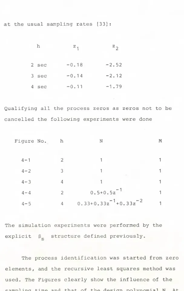
usual sampling rates [33] :

h Z 1 Z 2

2 sec -0.18 -2.52

3 sec -0.14 -2.12

4 sec -0.1 1 -1 .79

Qualifying all the process zeros as zeros not to cancelled the following experiments were done

Figure No. h N M

4-1 2 1 1

4-2 3 1 1

4-3 4 1 1

4-4 2 0.5+0.5z~1 1

4-5 4 0.33+0.33z_1+0.33z_2 1

The simulation experiments were performed by the explicit structure defined previously.

The process identification was started from zero elements, and the recursive least squares method was used. The Figures clearly show the influence of the sampling time and that of the design polynomial N. At the same time the fast convergence is also seen.

Figure 4-1.

y ( t )

i i

F i g u r e 4 - 2 .

Cd

■120 1~60 200 t [ s e c ]

F i g u r e 4 - 3 .

I

F i g u r e 4 - 4 .

u (t )

4

0 4 0 80 120 160

200

Figure 4-5.

- 73 -

REFERENCES

1. Allidina, A .Y . and Hughes, F . M . : Self-tuning Controller Steady-State Error.

Electronics Letters, V o l . 15, N o . 12, p p . 346-347, 1 979 .

2. Allidina, A.Y. and Hughes, F . M . : Generalized Self-tuning Controller with Pole Assignment. IEE P r o c . , Vol.

127, No. 1, pp. 13-18, 1980.

3. Allidina, A.Y. and Hughes, F . M . : A Generalized Minimum Variance Self-tuning Controller Incorporating Pole Assigment Specification. SOCOCO'82, Madrid.

4. Sström, K . J . : Introduction to stochastic control theory.

Academic Press, New York, 1970.

5. Xström, K.J. and Wittenmark, B . : On self-tuning regulators.

Automatica, Vol. 9, No. 2, pp. 185-199, 1973.

6. Sström, K.J. and Wittenmark,B.: Analysis of a Self-tuning Regulator for Nonminimum phase systems. IFAC,

Budapest, 1974.

7. Sström, K.J., W e s t e n b e r g ,B. and Wittenmark,B .: Self-

-tuning Controllers based on Pole-Placement Design.

Report of Lund Institute of Technology, Dept, of Aut. Control, (LUTED2/TFRT-3148), 1978.