Linear State Space Modeling and Control Teaching in MaxWhere Virtual Laboratory
Miklós Kuczmann, Tamás Budai
Széchenyi István University
Egyetem tér 1, H-9026 Győr, Hungary {kuczmann,budai.tamas}@sze.hu
Abstract: It is widely known that virtual laboratories can improve and complete university lectures. This paper presents laboratories, that allow engineering students to design a pole placement based controller for typical control problems: inverted pendulum, Furuta pendulum, crane, ball and beam. The dynamics of the plants and instructions for controller design and test are provided on smartboards of the virtual laboratory. The controller can be designed by the help of Octave Online. Finally, the controller performance can be studied by the model of the real-life application. The mathematical models and controller design are presented as well as the experiences in the virtual laboratory of control engineering.
Keywords: virtual laboratory; control engineering; pole placement
1 Introduction
Distance learning and e-Learning materials are widely used at universities worldwide. Virtual laboratories as special way of teaching and studying engineering disciplines provide interactive learning tools [1-12]. A virtual laboratory consists of an engineering system to be studied with supplementary learning materials like static texts, instructions, videos or different kinds of online software. This paper aiming at improving the lectures of Control Engineering [13- 15] by exercises that can be performed on typical model plants.
As and introductory example, Figure 1 shows a real-life Furuta pendulum [16] and its model in the MaxWhere framework [17]. To build up such a mechatronic system, it is necessary to design and develop the mechanics and the electronic part of the system. Furthermore, the informatic system is a central block to realize the controller, to actuate the motor and to collect measured sensor data and so on. In a control engineering laboratory, it is a challenging task to set up and to maintain all kinds of different mechatronic systems (e.g. different kinds of inverted
pendulums, crane, ball and beam system, liquid tank level, motors, vehicles, quadrotors, etc.) used every day by the students.
Introducing virtual laboratory with model equipment is an alternative fruitful way with many advantages [1-12, 18]. The students can study control in the frame of a homework collaborating with other students. All the learning materials suggested by the instructor are placed in the smartboards of the virtual laboratory. The labs are available to a wider audience worldwide. Professors can track student behavior and students can give feedback online. These labs are very cheap compared to the actual hardware.
There are some drawbacks [1-12, 18], indeed. There is a no hands-on contact with the real-life devices. The virtual laboratory cannot improve manual skills. It is difficult to sum up the situation in a real laboratory, anyway, virtual laboratory is safe. At the end, it is highlighted, that sophisticated mathematical models are necessary to represent a physical problem. It is noted that the MaxWhere framework already supports VR equipment which can help students to better immerse themselves into the virtual laboratory, but the overall efficiency must be studied by running a pilot laboratory with students. It can be concluded that virtual laboratories cannot substitute the real-life applications, but can improve the learning phase efficiently.
Control engineering is privilaged from the use of virtual laboratories, because every lecture note contain such typical instances like controlling the inverted pendulum, Furuta pendulum, crane, ball and beam, vehicles, liquid tank level, speed of a motor, and so on.
The venture of this work is to realize the model of typical plants used in the usual control engineering undergraduate lectures. Here, only pole placement is presented.
Figure 1
The hardware of a Furuta pendulum [16], and its model in the virtual control engineering lab
In the next section, the mathematical models and controller design are described shortly. Section 3 presents the virtual control engineering laboratory step-by-step.
Conclusions close the paper.
The proposed desktop client for the virtual control engineering laboratory is based on the MaxWhere framework [17]. MaxWhere is a unique engine for building 3D applications like the labs presented in this paper.
2 System Modeling and Control Design
2.1 State Space Model
The Euler-Lagrange equations [13-15]
d d𝑡
𝜕𝐾
𝜕𝑞̇𝑖−𝜕𝑞𝜕𝐾
𝑖+𝜕𝑞𝜕𝑃
𝑖+𝜕𝑞̇𝜕𝑅
𝑖= 𝜏𝑖 (1)
have been applied to set up the dynamic model of the mentioned plants to be controlled. In (1) K, Pand R are the kinetic energy, the potential energy, the Rayleigh term for friction, qi and 𝜏𝑖 are the generalized coordinates and the generalized torque or force, respectively. All the presented systems have two degrees of freedom, i.e. i=1,2.
The control signal is the input of the plant (force or torque), generally denoted by u.
2.1.1 The Inverted Pendulum
The inverted pendulum, shown in Figure 2, simply falls over if the cart is not moved to balance it, i.e. the control aim is to balance the pendulum, or in other words, to reach a state where the inclination angle 𝜑is zero.
The kinetic and potential energy of the inverted pendulum are described by the equations [19, 20]
𝐾 =12𝑚𝑥̇2+12𝑀𝑣𝑀2 +12𝑚𝑠𝑣𝑠2+12𝐼𝜑̇2, (2)
𝑃 = 𝑀𝑔𝐿𝐶𝜑+ 𝑚𝑠𝑔𝑙𝐶𝜑, (3)
containing the length and mass of the rod 2L, and M, the position and mass of the sphere l and ms, the mass of the cart m, the moment of inertia of the rod 𝐼 =
1
3𝑀𝐿2, and finally, the gravitational acceleration g. The state variables are the position x and the speed 𝑥̇ of the cart, moreover the inclination angle and speed of the rod denoted by 𝜑 and 𝜑̇, respectively. For simplicity the following notations
are used: 𝑆𝜑= sin𝜑 and 𝐶𝜑= cos𝜑. The velocity of the center of mass of the rod as well as the sphere,𝑣𝑀 and 𝑣𝑠, are derived by the state variables. Friction has not taken into account in this model, i.e. 𝑅 = 0.
The nonlinear state space model of the inverted pendulum can be obtained by deriving (1) with (2) and (3). It is highlighted that the simulation of the system is performed by the nonlinear model. However, the controller is designed by the linearized model.
The details of setting up the mathematical description can be found in [19].
Figure 2
The inverted pendulum model
The linearized state space model of the inverted pendulumin the unstable upright position is as follows:
[ 𝑥̇
𝑥̈
𝜑̇
𝜑̈
] = [
0 1 0 0 0 0 𝑞 0 0 0 0 1 0 0 𝑝2 0
] [ 𝑥𝑥̇
𝜑 𝜑̇
] + [ 𝛽0 0 𝛼
] 𝑢, (4)
where q, p, 𝛼 and 𝛽 are model parameters.
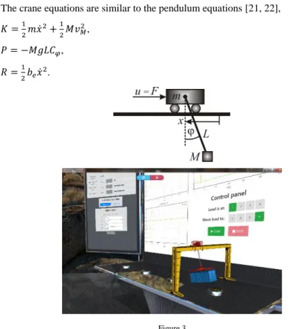
2.1.2 The Crane
The gantry crane is a transportation system of heavy loads, presented in Figure 3.
The control goal is to reach accurate positioning of payloads.
The crane equations are similar to the pendulum equations [21, 22],
𝐾 =12𝑚𝑥̇2+12𝑀𝑣𝑀2, (5)
𝑃 = −𝑀𝑔𝐿𝐶𝜑, (6)
𝑅 =12𝑏𝑒𝑥̇2. (7)
Figure 3 The crane model
The friction of the cart along the x axis has been taken into account by the linear model of friction with the parameter be in (7).
The nonlinear state space model of the crane has been derived by (1) with (5)-(7).
The state space model of the system can be linearized in the stable downward position:
[ 𝑥̇
𝜑̇𝑥̈
𝜑̈
] = [
0 1 0 0 0 𝑎 𝑏 0 0 0 0 1 0 𝑐 𝑑 0
] [ 𝑥𝑥̇
𝜑 𝜑̇
] + [ 𝛽0 0 𝛼
] 𝑢. (8)
Here, a, b, c, d, moreover 𝛼 and 𝛽 are model parameters. The details are presented in [21, 22].
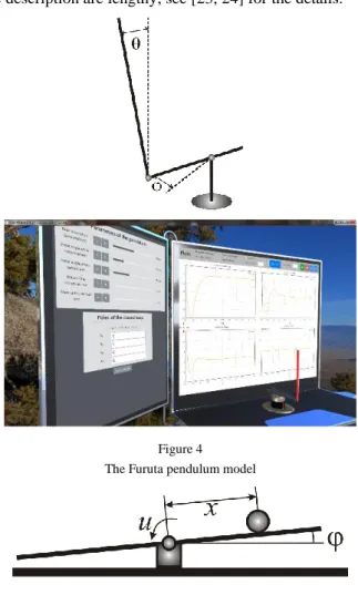
2.1.3 The Furuta Pendulum
The Furuta pendulum is another kind of the inverted pendulum, shown in Figure 4. The control aim is again, to balance the pendulum.
The equations of the Furuta pendulum are tedious, deriving the energy terms and the state space description are lengthy, see [23, 24] for the details.
Figure 4 The Furuta pendulum model
Figure 5
The model of ball and beam system
The linearized state space model of the Furuta pendulum at the unstable upright position is as follows:
[ 𝜑̇
𝜑̈
𝜃̇
𝜃̈
] = [
0 1 0 0 0 0 𝛿 0 0 0 0 1 0 0 𝛾 0
] [ 𝜑 𝜑̇
𝜃 𝜃̇
] + [ 𝛽0 0 𝛼
] 𝑢. (9)
Here, 𝛿, 𝛾, 𝛼, and 𝛽 are model parameters.
2.1.4 The Ball and Beam System
The ball and beam system can be seen in Figure 5. Here, the aim is to balance a ball on a beam by appropriate control signal.
The linearized state space model of the ball and beam system are as follows:
[ 𝑥̇
𝑥̈
𝜑̇
𝜑̈
] = [
0 1 0 0 0 0 𝑎 0 0 0 0 1 0 0 0 0
] [ 𝑥𝑥̇
𝜑 𝜑̇
] + [ 0 00 𝛼
] 𝑢, (10)
where, a and 𝛼 are model parameters. See [24] for the detailed description.
2.2 Pole Placement Design
The above mentioned systems have the same form [13-15, 25, 26]
𝐱̇ = 𝐀𝐱 + 𝐛𝑢, (11)
where A is the system matrix which eigenvalues determine the stability and performance of the open loop system, x is the state vector, b is a column vector and u is the acting input.
The input signal is a pushing-pulling force in the case of the pendulum and crane, but it is torque for the Furuta pendulum and for the ball and beam system. Force and torque are supplied by electric motors in the real-life applications, anyway, for making the models as simple as possible, the actuators are not modeled in these laboratories.
Control has been performed by pole placement technique [13-15, 25, 26]. The control signal u is defined by (Figure 6)
𝑢 = −𝐤T𝐱 = −𝑘1𝑥1− 𝑘2𝑥2− 𝑘3𝑥3− 𝑘4𝑥4, (12) i.e. the control signal is the weighted sum of the state variables. The controller parameters 𝐤T= [𝑘1 𝑘2 𝑘3 𝑘4] can be designed as follows:
Figure 6
The pole placement based control system
The eigenvalues of A can be obtained by the characteristic equation
𝜑o(𝜆) = |𝜆𝐈4x4− 𝐀| = 𝜆4+ 𝑎1𝜆3+ 𝑎2𝜆2+ 𝑎3𝜆 + 𝑎4= 0, (13) where 𝐈4x4 is the 4x4 identity matrix, the coefficients a1, a2, a3, a4 are known, the subscript o is for the open loop system. The transient behavior is determined by the eigenvalues 𝜆, and this behavior can be modified by the state feedback. On one hand, some of the eigenvalues are zero or live on the right hand side of the complex plane resulting in an unstable system, like the pendulums as well as the ball and beam system. These systems must be stabilized at least, i.e. the unwanted eigenvalues must be placed to the left hand side of the complex plane. On the other hand, the system is stable (the crane) with inconvenient and slow transient behavior, which can be changed by simply designing new eigenvalues for the closed loop system.
The feedback modifies the system matrix by a diad as follows:
𝐱̇ = 𝐀𝐱 + 𝐛𝑢 = (𝐀 − 𝐛𝐤T)𝐱. (14)
The desired eigenvalues of the closed loop system can be set according to 𝜑cl(𝜆) = |𝜆𝐈4x4− (𝐀 − 𝐛𝐤T)| = (𝜆 − 𝜆1)(𝜆 − 𝜆2)(𝜆 − 𝜆3)(𝜆 − 𝜆4)
= 𝜆4+ 𝑝1𝜆3+ 𝑝2𝜆2+ 𝑝3𝜆 + 𝑝4= 0, (15)
where the coefficients p1, p2, p3, p4 are determined by the desired eigenvalues 𝜆1, 𝜆2, 𝜆3, 𝜆4 for which the feedback gains can be designed by the Ackermann’s formula:
𝐤T= [0 0 0 1]𝐌c−1𝜑cl(𝐀). (16)
Here, the matrix 𝐌c is essential, called the controllability matrix, set up as
𝐌c = [𝐛 𝐀𝐛 𝐀2𝐛 𝐀3𝐛], (17)
which rank must be maximum, i.e. rank𝐌c = 4, otherwise the inverse cannot be computed in (16). These kinds of systems are called controllable system. The last term in (16) is computed as follows
𝜑cl(𝐀) = 𝐀4+ 𝑝1𝐀3+ 𝑝2𝐀2+ 𝑝3𝐀 + 𝑝4𝐈4x4. (18) In Octave [27], pole placement can be performed by the command place.
3 Control Engineering in MaxWhere
The above-mentioned system models and pole placement based controller design has been implemented in MaxWhere [17].
The virtual laboratories are able to present the behavior of the nonlinear system model as well as linear controller design, finally the designed controller can be checked by the virtual system model. An example is shown in Figure 7, the crane model is on the table put on the right, learning materials and Octave Online are situated on the left hand side.
Figure 7
A typical control laboratory with web pages and the equipment
The learning material is shown in Figure 8. There are four smartboards containing the text in pdf.
The first board shows the model and the state space representation, but not in detail.
The second board presents the block diagram and the main idea of the closed loop system with the controller.
There are two exercises highlighted on the last two boards. On the first one, the effect of eigenvalues can be explored by changing the desired eigenvalues in (15).
The relationship between eigenvalues and state variables is an instructive experiment for the students. Second, the controller gains are designed by the provided Octave code (see Figure 9), than the designed controller can be tested as it is shown by Figure 10. The Octave Online is applicable to study the model set up, the eigenvalues, the impulse response of the open loop as well as the designed closed loop system. This task is very useful for the students because they can study the syntax of Octave and its toolboxes.
It is noted, that the smartboard materials can be replaced easily by the lecturer, also it is important to mention that any web-based tool (like Octave Online in this example) can be used in all smartboards.
Figure 8
Web pages of learning material for crane model and control
Figure 9
Running controller design and test in Octave Online
Figure 10
Testing the linear controller on the nonlinear system of crane
Conclusions
Virtual control engineering laboratories have been designed to supplement traditional undergraduate lectures. Modeling methodology and pole placement based controller design technique can be studied and practised.
The next step is to broaden the assortment of available systems, as well as to realize other types of controllers.
The four gains of the controller can be designed by other techniques in these labs.
For example, implementing linear quadratic regulator (LQR) is very easy by
replacing the command place with lqr. There are many other potentials in the virtual word that will be discovered with the help of tutors and students.
Acknowledgement
This work was supported by the FIEK program (Center for cooperation between higher education and the industries at the Széchenyi István University, GINOP- 2.3.4-15-2016-00003)
References
[1] V. Potkonjak, M. Gardner, V. Callaghan, P.Mattila, C. Guetl, V. M.
Petrović, K. Jovanović. Virtual laboratories for education in science, technology, and engineering: A review. Computers & Education, Vol. 95, 2016, pp. 309-327
[2] T. Budai, M. Kuczmann. Towards a modern, integrated virtual laboratory system. Acta Polytechnica Hungarica, Vol. 15, No. 3, 2018, pp. 191-204 [3] B. Berki. Desktop VR as a Virtual Workspace: a Cognitive Aspect. Acta
Polytechnica Hungarica, Vol. 16, No. 2, 2019, pp. 219-231
[4] I. Horváth. MaxWhere 3D capabilities contributing to the Enhanced Performance of Trello 2D software. Acta Polytechnica Hungarica, 2019, in print
[5] B. Berki. 2D Advertising in 3D Virtual Spaces. Acta Polytechnica Hungarica, Vol. 15, No. 3, 2018, pp. 175-190
[6] I. Horváth, A. Sudár. Factors Contributing to the Enhanced Performance of the MaxWhere 3D VR Platform in the Distribution of Digital Information.
Acta Polytechnica Hungarica, Vol. 15, No. 3, 2018, pp. 149-173
[7] B. Lampert, A. Pongrácz, J. Sipos, A. Vehrer, I. Horvath. MaxWhere VR- learning improves effectiveness over clasiccal tools of e-learning. Acta Polytechnica Hungarica, Vol. 15, No. 3, 2018, pp. 125-147
[8] B. Berki. Better Memory Performance for Images in MaxWhere 3D VR Space than in Website, 9th IEEE International Conference on Cognitive Infocommunications CogInfoCom, 2018, pp. 283-287
[9] I. Horváth. Evolution of teaching roles and tasks in VR/AR-based education In Cognitive Infocommunications (CogInfoCom) 9th IEEE International Conference, Budapest, 2018
[10] A. Csapo, I. Horváth, P. Galambos, P. Baranyi. VR as a Medium of Communication: from Memory Palaces to Comprehensive Memory Management In Cognitive Infocommunications (CogInfoCom) 9th IEEE International Conference, Budapest, 2018
[11] P. Baranyi, A. Csapo, Gy. Sallai. Cognitive Infocommunications (CogInfoCom) Springer, 2015
[12] P. Baranyi, A. Csapó. Definition and synergies of cognitive infocommunications. Acta Polytechnica Hungarica, Vol. 9, No. 1, 2012, pp.
67-83
[13] L. Keviczky, R. Bars, J. Hetthéssy, C. Bányász. Control engineering. 2019, Springer
[14] B. Lantos. Control systems, theory and design I. 2009, Academic Press, Budapest
[15] J. Bokor, P. Gáspár. Control engineering with vehicle dynamic applications. 2008, TypoTex, Budapest
[16] Rotary Inverted Pendulum. http://www.quanser.com/products/rotary _pendulum [online, last visited on: 2019.06.06]
[17] MaxWhere website. https://www.maxwhere.com/ [online, last visited on:
2019.06.06]
[18] I. Horváth. Innovative engineering education inthe cooperative VR environment. Proceedings of the 7th IEEE Conference on Cognitive Infocommunications. Wrocław, Poland, 2016
[19] M. Kuczmann. State space based linear controller design for the inverted pendulum. Acta Technica Jaurinensis, Vol. 12, No. 2, 2019, pp. 130-147 [20] P. Gáspár, J. Bokor, A. Soumelidis. An inverted pendulum tool for teaching
linear optimal and model based control. Periodica Polytechnica Transportation Engineering, Vol. 25, No. 1-2, 1997, pp. 9-19
[21] N. M. Bashir, A. A. Bature, A. M. Abdullahi. Pole placement control of a 2D gantry crane system with varying pole locations. Applications of Modelling and Simulation, Vol. 2, No. 1, 2018, pp. 8-16
[22] G. Bartolini, A. Pisano, E. Usai. Output-feedback control of container cranes: a comparative analysis. Asian Journal of Control, Vol. 5, No. 4, 2003, pp. 578-593
[23] B. S. Cazzolato, Z. Prime. On the dynamics of the Furuta pendulum.
Journal of Control Science and Engineering, Vol. 2011, Article ID: 528341, 2011
[24] K. Haga, P. Ratiroch-Anant, H. Hirata, M. Anabuki, S. Ouchi. Self-tuning control for totation type inverted pendulum using two kinds of adaptive controllers. IEEE Conference on Robotics, Automation and Mechatronics, 2006
[25] K. Ogata. Modern control engineering. Prentice-Hall, 1997
[26] K. J. Aström, R. M. Murray. Feedback systems: an introduction for scientists and engineers. Princeton University Press, 2008
[27] Octave Online. https://octave-online.net/ [online, last visited on:
2019.06.06]