Two-Area Power System Stability Improvement using a Robust Controller-based CSC-STATCOM

Two-Area Power System Stability Improvement using a Robust Controller-based CSC-

STATCOM

Sandeep Gupta, Ramesh Kumar Tripathi

Department of Electrical Engineering

Motilal Nehru National Institute of Technology Allahabad - 211004, India E-mail: ree0951@mnnit.ac.in, rktripathi@mnnit.ac.in

Abstract: A current source converter (CSC) based static synchronous compensator (STATCOM) is a shunt flexible AC transmission system (FACTS) device, which has a vital role in stability support for transient instability and damping support for undesirable inter- area oscillations in an interconnected power network. A robust pole-shifting based controller for CSC-STATCOM with damping stabilizer is proposed. In this paper, pole- shifting controller based CSC-STATCOM is designed for enhancing the transient stability of two-area power system and PSS based damping stabilizer is designed to improve the oscillation damping ability. First of all, modeling and pole-shifting based controller design, with damping stabilizer for CSC-STATCOM, are described. Then, the impact of the proposed scheme in a test system with different disturbances is demonstrated. The feasibility of the proposed scheme is demonstrated through simulation in MATLAB and the simulation results show an improvement in power system stability in terms of transient stability and oscillation damping ability with damping stabilizer based CSC-STATCOM. So good coordination between damping stabilizer and pole-shifting controller based CSC- STATCOM is shown in this paper for enhancing the power system stability. Moreover, the robustness and effectiveness of the proposed control scheme are better than without damping stabilizer in CSC-STATCOM.

Keywords: CSC; PSS; STATCOM; transient stability; oscillation damping

1 Introduction

The continuous enhancement of electrical loads due to the growing industrialization and modernization of human activity results in transmission structures being operated near their stability restrictions. Therefore, the renovation of urban and rural power network becomes necessary. Due to governmental, financial and green climate reasons, it is not always possible to construct new transmission lines to relieve the power system stability problem for existing overloaded transmission lines. As a result, the utility industry is facing the

challenge of efficient utilization of the existing AC transmission lines in power system networks. So transient stability, voltage regulation, damping oscillations etc. are the most important operating issues that electrical engineers face during power-transfer at high levels.

In the above mentioned power quality problems, transient stability and oscillation damping are the two most important factors during power-transfer at high levels.

According to the literature, transient stability of a power system is its ability to maintain synchronous operation of machines, when subjected to a large disturbance [1]. And oscillation damping is the positive damping of electromechanical modes or oscillations among the interconnected synchronous generators in a power system [2]. While the generator excitation system with PSS (power system stabilizer) can maintain excitation control and stability, but it is not adequate to sustain the stability of power system due to faults or overloading near to the generator terminals [1]. Therefore, researchers have been working on this problem for a long time trying to discover a solution. One of the powerful methods for enhancing the transient stability is to use flexible AC transmission system (FACTS) devices [3-5]. But oscillation damping is improved by the use of damping stabilizer [6]. So power system stability is increased with the help of damping stabilizer (PSS) based FACTS devices [7-9]. Even though the prime objective of shunt FACTS devices (SVC, STATCOM) is to maintain bus voltage by absorbing (or injecting) reactive power, they are also competent of improving the system stability by diminishing (or enhancing) the capability of power transfer when the machine angle decreases (increases), which is accomplished by operating the shunt FACTS devices in inductive (capacitive) mode.

In the cited research papers [4, 7, 10-13], different types of these devices and/or damping stabilizer with different control techniques are used for improving transient stability & enhancing oscillation damping. In these, researchers have investigated the co-ordination of PSS and FACTS based controller [7, 11, 13]. So the PSS based FACTS devices are playing an important role for improving the oscillation damping with transient stability. Among these FACTS devices, the STATCOM is valuable for enhancement of power system dynamic stability and frequency stabilization due to the rapid output response, lower harmonics, superior control stability and small size etc. [14]. By their inverter configuration, basic type of STATCOM topology can be realized by either a current-source converter (CSC) or a voltage-source converter (VSC) [14, 15]. But recent research confirms several advantages of CSC based STATCOM over VSC based STATCOM [16, 17]. These advantages are high converter reliability, quick starting, inherent short-circuit protection, the output current of the converter is directly controlled, in low switching frequency this reduces the filtering requirements compared with the case of a VSC. Therefore CSC based STATCOM is very useful in power systems rather than VSC based STATCOM in many cases.

Hence, coordination of PSS and CSC-STATCOM can be used for enhancement of power system dynamic stability.

Presently, the most used techniques for controller design of FACTS devices are Proportional Integration (PI) [12], PID controller, pole placement and linear quadratic regulator (LQR) [18]. But, LQR and pole placement algorithms give quicker response in comparison to PI & PID algorithm. LQR controller Gain (K) can be calculated by solving the Riccati equation and K is also dependent on the two cost function (Q, R). So Riccati equation solvers have some limitations, which relate to the input arguments. But pole shifting method does not face this type of problem. So pole shifting method gives a better and robust performance in comparison to other methods.

The main contribution of this paper is the application of proposed pole-shifting controller based CSC-STATCOM with damping stabilizer for improvement of power system dynamic stability (in terms of transient stability and oscillation damping) by injecting (or absorbing) reactive power. In this paper, the proposed scheme is used in two-area power system with dynamic loads under a severe disturbance (three phase fault or heavy loading) to enhance the power system stability and observe the impact of the CSC-based STATCOM on electromechanical oscillations and transmission capacity. Further, the results obtained from the proposed algorithm-based CSC-STATCOM are compared to that obtained from the conventional methods (without CSC-STATCOM device and without damping stabilizer in CSC-STATCOM).

The rest of the paper is organized as follows. Section 2 discusses the circuit modeling & pole-shifting controller design for CSC based STATCOM. A two- area tow-machine power system is described with a CSC-STATCOM device in Section 3. Coordinated design of pole-shifting based CSC-STATCOM with Damping Stabilizer is proposed in Section 4. Simulation results, to improve power system dynamic stability of the test system with & without CSC based STATCOM (and/or damping stabilizer) for severe contingency are shown in Section 5. Finally, Section 6 concludes this paper.

2 Mathematical Modeling of Pole-shifting Controller- based CSC-STATCOM

2.1 CSC-based STATCOM Model

To verify the response of the CSC-based STATCOM on dynamic performance, the mathematical modeling and control strategy of a CSC-based STATCOM are presented. The design of controller for CSC based STATCOM, the state space equations from the CSC-STATCOM circuit are introduced. To minimize the complexity of mathematical calculations, the theory of dq transformation of

currents has been applied in this circuit, which makes the d and q components as independent parameters. Figure 1 shows the circuit diagram of a typical CSC- based STATCOM.

Figure 1

The representation of CSC based STATCOM

Where

i_SR, i_SS, i_ST line current

v_CR, v_CS, v_CT voltages across the filter capacitors v_R, v_S, v_T line voltages

I_dc dc-side current

R_dC converter switching and conduction losses L_dc smoothing inductor

L inductance of the line reactor R resistance of the line reactor

C filter capacitance

The basic mathematical equations of the CSC-STATCOM have been derived in the literature [17]. Therefore, only a brief detail of the test-system is given here for the readers’ convenience. Based on the equivalent circuit of CSC-STATCOM shown in Figure 1, the differential equations for the system can be achieved, which are derived in the abc frame and then transformed into the synchronous dq frame using dq transformation method [19].

3 3

- - -

2 2

d Idc Rdc Idc M Vd d M Vq q

dt Ldc Ldc Ldc

 (1)

1 1

- - E

d Id RId Iq d Vd

dt  L  L n L (2)

- - 1

d R

Iq Id Iq Vq

dt   L L (3)

Real power flow

Area-1 Area-2

Sending end Receiving end

a b c

Idc

iR

R L

C

Ldc,Rdc

vCR

vCS

vCT

S₁ S3

S2 S4

S5

S6

v_R vS

vT

iSS

iST

iSR

iS

iT

iCR Transformer

CSC-STATCOM

1 1 d -

Vd Id Vq M Id dc

dt  C  C (4)

1 1

- -

dVq Iq Vd M Iq dc

dt  C  C (5)

In above differential equations M_d and M_q are the two input variables. Two output variables are I_dc and I_q. Here, ω is the rotation frequency of the system and this is equal to the nominal frequency of the system voltage. Equations (1 to 5) show that controller for CSC based STATCOM has a nonlinear characteristic. So this nonlinear property can be removed by accurately modeling of CSC based STATCOM. From equations (1 to 5), we can see that nonlinear property in the CSC-STATCOM model is due to the part of I_dc. This nonlinear property is removed with the help of active power balance equation. Here, we have assumed that the power loss in the switches and resistance R_dc is ignored in this system and the turns ratio of the shunt transformer is n:1. After using power balance equation and mathematical calculation, nonlinear characteristic is removed from equation (1). Finally we obtain the equation as below:

 

 

d Idc dc Idc d Id

dt Ldc Ldcn

 (6)

In the equation (6) state variable (I_dc) is replaced by the state variable (I²_dc), to make the dynamic equation linear. Finally, the better dynamic and robust model of the SATACOM in matrix form can be derived as:

   

2 3

- 0 0 0

0 0

2 2

1 0 0

0 - 0

0 0

1 * 1 *

0 - - 0

0

1 1

0 - 0 0

0

0 0 -1 - 0

Rdc Ed Ldc Ldcn

idc R idc

L o L

id id I

d R id

iq o iq I

dt L L iq

vcd vcd C

vcq C o vcq C

C o









 

 

   

       

       

       

        

     

       

       

       

     

       

 

 

0 -1

0 * 0 0

L Ed

 

 

 

  

    

   

 

 

 

 

(7) Above modeling of CSC based STATCOM is written in the form of modern control methods i.e. State-space representation. For state-space modeling of the system, section 2.2 is considered.

2.2 Pole-Shifting Controller Design

The pole-shift technique is one of the basic control methods employed in feedback control system theory. Theoretically, Pole shift technique is to set the preferred pole position and to move the pole position of the system to that preferred pole position, to get the desired system outcomes [20]. Here poles of system are shifted because the position of the poles related directly to the eigenvalues of the system, which control the dynamic characteristics of the system outcomes. But for this method, the system must be controllable. In the dynamic modeling of systems, State-space equations involve three types of variables: state variables (x), input(u) and output (y) variables with disturbance (e). So comparing (7) with the standard state-space representation i.e.

xAx Bu Fe (8)

yCx (9)

We get the system matrices as:

2 T

x Idc Id Iq Vd Vq ^;

u Iid IiqT^; eEd; 2 T y Idc Iq

2 3

- - 0 0 0

0 - 1 0

0 - - 0 1

0 -1 0 0

0 0 -1 - 0

Rdc Ed Ldc Ldc R

L L

A R

L L

c c









 

 

 

 

 

 

 

  

 

 

 

 

 

 

 

;

0 0 0 0 0 0 1 0 0 1 B

c c



 

 

 

 

 

 

 

 

 

 

;

1 0 0 0 0 1 0 0 0 0

T

C

 

 

 

 

 

 

 

 

; 0 -1

0 0 0 F L

 

 

 

 

  

 

 

 

 

In above equations (8, 9) five system states, two control inputs and two control outputs are presented. Where x is the state vector, u is the input vector, A is the basis matrix, B is the input matrix, e is disturbance input.

If the controller is set as:

-

u Kx Ty ref Me (10)

Then the state equation of closed loop can be written as

( - )

x A BK x Ty ref BMeFe (11)

Where T=(C*(-(A-B*K)-1)*B)-1 and M= ((C* (-A+B*K)-1*B))-1*(C*(-A+B*K)- 1*F), these values are find out from mathematical calculation. Here K is the state- feedback gain matrix. The gain matrix K is designed in such a way that equation (12) is satisfied with the desired poles.

- ( - ) ( - 1)( - 2)...( - )

sI A BK  s P s P s Pn (12)

Where P₁, P₂, …..Pn are the desired pole locations. Equation (12) is the desired characteristic polynomial equation. The values of P₁, P₂, …..Pn are selected such as the system becomes stable and all closed-loop eigenvalues are located in the left half of the complex-plane. The final configuration of the proposed pole- shifting controller based CSC-STATCOM is shown in Figure 2.

B ∫dt C

A -K

x X y

u

M* F* Ed

Output Responses for Two Area Power System

CSC- STATCOM Ldc

Rdc

T*yref

Ed

Pole-shifting Controller

Figure 2

Control Structure of pole-shifting controller based CSC-STATCOM

3 Two-Area Power System with CSC-STATCOM FACTS Device

Real power flow

Area-1 Area-2

L1 L2

Sending end Receiving end

E1 Vb E2

a b c

E1 δ E2 0°

Icsc

jX1 jX2

Vb θb

CSC based STATCOM device

Figure 3

A single line diagram of two-area two-machine power system with CSC-STATCOM

Firstly consider a two-area two-machine power system with a CSC-STATCOM at bus b is connected through a long transmission system, where CSC-STATCOM is used as a shunt current source device. Figure 3 shows this representation. The

dynamic model of the machine, with a CSC-STATCOM, can be written in the differential algebraic equation form as follows:

 

1 csc

m eo

P P Pe

M



 

 

Here ω is the rotor speed, δ is the rotor angle, Pm is the mechanical input power of generator, the output electrical power without CSC-STATCOM is represents by P_eo and M is the moment of inertia of the rotor. Equation (14) is also called the

“swing equation”. The additional factor of the output electrical power of generator from a CSC-STATCOM is P_e^csc in the swing equation. Here for calculation of P_e^csc, to assume the CSC-STATCOM works in capacitive mode. Then the injected current from CSC-STATCOM to test system can be written as:

( 90 )

csc csc o

I I bo (15)

Where, θbo is the voltage angle at bus b in absentia of CSC-STATCOM. In Figure 3, the magnitude (Vb) and angle (θb) of voltage at bus b can be computed as:

1 2 1sin

tan 2 1cos 1 2

X E

b X E X E

 



 

   

  

  (16)

cos( ) cos

2 1 1 2 1 2

csc

1 2 1 2

X E bo X E bo X X

Vb X X X X I

  

     

        (17)

From equation (17), it can be said that the voltage magnitude of bus b (V_b) depends on the STATCOM current I_csc. In equation (14), the electrical output power P_e^csc of machine due to a CSC-STATCOM, can be expressed as

csc 1 sin( )

1 E Vb

Pe b

X

 

  (18)

Finally, using equations (17) & (18) the total electrical output (Pe) of machine with CSC-STATCOM can be written as

csc 1 2 1 cscsin( )

( 1 2) 1 X X E

PePeoPe  PePeo X X X I   b

 (19)

All above equations are represented for the capacitive mode of CSC-STATCOM.

For the inductive mode of operation negative value of I_csc can be substituted in equations (15), (17) & (19) in place of positive I_csc. With the help of equation (14), the power-angle curve of the test system can be drawn for stability analysis as shown in Figure 4.

a

b c d e

f

g

δ0 δc δm

0

Prefault Curve A Pe (Icsc = 0) Postfault Curve C

Pe p (I_csc > 0)

Fault duration Curve B, Pe

f

Postfault Curve C (I_csc < 0)

Ad

Aa P_m

Figure 4

Power-angle characteristic of the test system with a CSC-STATCOM

The power-angle (P-δ) curve of the test system without a CSC-STATCOM is represented by curve A (also called Prefault condition) in Figure 4. Here the mechanical input is P_m, electrical output is P_e and initial angle is δ₀. When a fault occurs, P_e suddenly decreases and the operation shifts from point a to point b on curve B, and thus, the machine accelerates from point b to point c, where accelerating power P_a [= (P_m-P_e)] >0. At fault clearing, P_e suddenly increases and the area a-b-c-d-a represents the accelerating area A_a as defined in equation (20).

If the CSC-STATCOM operates in a capacitive mode (at fault clearing), P_e increases to point e at curve C (also called postfault condition). At this time P_a is negative. Thus the machine starts decelerating but its angle continues to increase from point e to the point f until reaches a maximum allowable value δ_m at point f, for system stability. The area e-f-g-d-e represents the decelerating area A_d as defined in equation (20). From previous literature [1], equal area criterion for stability of the system can be written as:

  ^{ }

0

f p

c Pm Pe d cm Pe Pm d Aa Ad

   

 ^{ }  ^{  }

  ⁽²⁰⁾

This equation is generated from Figure 4, where δ_c is critical clearing angle. P_e^p is an electrical output for post-fault condition. P_e^f is an electrical output during fault condition. From Figure 4, it is seen that for capacitive mode of operation (I_csc>0), the P-δ curve is not only uplifted but also displaced toward right and that endues more decelerating area and hence higher transient stability limit. But pole-shifting controller based CSC-STATCOM is not given to sufficient oscillation damping stability. So additional controller with pole-shifting controller based CSC- STATCOM is essential for oscillation damping in the power system. The additional controller is detailed in the next section.

4 Coordinated Design of Pole-Shifting Controller- based CSC-STATCOM with Damping Stabilizer

In this section, a damping stabilizer with pole-shifting controller is proposed for CSC-STATCOM to improve the oscillation damping and transient stability of the system. Modeling of a pole-shifting controller based CSC-STATCOM is explained earlier in section 2.2. So design of a damping stabilizer for pole-shifting controller based CSC-STATCOM is explained in this section. Here PSS-based damping controller is used for damping stabilizer designing. The basic function of power system stabilizer (PSS) is to add damping to the generator rotor oscillations by controlling its excitation using auxiliary stabilizing signals [6]. These auxiliary signals are such as shaft speed, terminal frequency and power to change and adding these output signals of damping stabilizer with a reference signal of pole- shifting controller based CSC-STATCOM. Here coordination between PSS-based damping stabilizer and pole-shifting controller based CSC-STATCOM is very necessary and important.

Output Responses for Two-area power

system Pole-shifting

controller based CSC-STATCOM

I

V

V

V

Δω

(input signal)

y

Washout Gain Compensator

Damping Stabilizer Vs(min)

Vs(max)

y

Iq(ref)

  

  

  

  

1+sT 1+sT

3 1

1+sT 1+sT

4 2

 

 

 

 

sTw 1+Tw

Ks

Figure 5

Configuration of damping stabilizer for pole-shifting controller-based CSC-STATCOM

So the damping stabilizer is designed carefully with respect to pole-shifting controller based CSC-STATCOM. A typical structure of damping stabilizer is taken as shown in Figure 5. In this paper, IEEE ST1-Type excitation based PSS is used [1]. The damping stabilizer structure contains one washout block, one gain block and lead-lag compensation block. The number of lead-lag blocks required depends on the power system configuration and PSS tuning. Here the washout block works like as a high pass filter which removes low frequencies from the input signal of the damping stabilizer. The ability of phase lead-lag compensation block is to give the required phase-lead characteristics to compensate for any phase lag between the input and the output signals of damping stabilizer. Hence, transfer function of the damping stabilizer is obtained as follows:

1 3 1 1

1 1 4 1 2

sT sT

Sout Ks sTw Sin

Tw sT sT

 

   

  

 

  

 

   

Where S_in is the damping stabilizer input signal. S_out is the damping stabilizer output signal. K_s is the PSS gain. T_w is the washout time constant. T₁, T₂, T₃, T₄ are the compensator time constants. In this arrangement T_w, T₂ and T₄ are generally predefined values. The value of washout time constant (T_w) is not critical issue and may be in the range 1–20 s [1]. The PSS gain K_s and values of T₁

& T₂ are to be found from simulation results and some previous Artificial intelligence techniques based papers [21, 22]. In Figure 5, V_s(max) & V_s(min) are the maximum & minimum values of damping stabilizer respectively which are predefined values for the test-system. Hence, all the data required for designing of damping stabilizer based controller are given in Appendix 1. In this paper, the input signal of the proposed PSS based damping stabilizer is the rotor speed deviation of two machines (M1 & M2), Δω = ω1 - ω2, which is mentioned in equations (13) & (14). Now in the following section the test-system stability in terms of transient stability and oscillations damping ability is analyzed and enhanced using the proposed damping stabilizer based pole-shifting controller with CSC-STATCOM.

5 Simulation Results

5.1 Power System under Study

Excitation System

Generator

Turbine & governor

system Excitation

System

Generator

Turbine & governor system

CSC-STATCOM Ldc Rdc

Large load center (5000MW)

1 0.95

Hydraulic power plant (P1) Hydraulic power plant (P2)

Vref P_ref1

1 0.81

Vref Pref2

1000 MVA 13.8 kV/500 kV

5000 MVA 13.8 kV/500 kV

Three phase Fault

(Case I) Heavy Loading (Case II)

950 MW 4050 MW

B1 B2 B3

L1 (350 km)

L2 (350 km)

Machine 1 Machine 2

(M1) (M2)

Figure 6

The single line diagram of the test-system model for power system stability study of two power plants (P1 & P2)

In this section, two-area power system is considered as a test system for study. For this type of test system, a 500kV transmission system with two hydraulic power plants P₁ (machine-1) & P₂ (machine-2) connected through a 700 km long transmission line is used, as shown in Figure 6. Rating of first power generation plant (P1) is 13.8 kv/1000 MVA, which is used as PV generator bus type. The electrical output of the second power plant (P2) is 5000 MVA, which is used as a swing bus for balancing the power. One 5000 MW large resistive load is connected near the plant P2 as shown in Figure 6. To improve the transient stability and increase the oscillation damping ability of the test-system after disturbances (faults or heavy loading), a pole-shifting controller based CSC- STATCOM with damping stabilizer is connected at the mid-point of transmission line. To achieve maximum efficiency; CSC-STATCOM is connected at the mid- point of transmission line, as per [23]. The two hydraulic generating units are assembled with a turbine-governor set and excitation system, as explained in [1].

All the data required for this test system model are given in Appendix 1.

The impact of the damping stabilizer based CSC-STATCOM has been observed for maintaining the system stability through MATLAB/SIMULINK. Severe contingencies, such as short-circuit fault and instant loading, are considered.

5.2 Case I—Short-Circuit Fault

A three-phase fault is created near bus B1 at t=0.1 s and is cleared at 0.23 s. The impact of system with & without CSC based STATCOM (and/or damping stabilizer) to this disturbance is shown in Figures 7 to 14. Here simulations are carried out for 9 s to observe the nature of transients. From Figures 7 to 10, it is observed that the system without CSC-STATCOM is unstable even after the clearance of the fault. But this system with pole-shifting controller based CSC- STATCOM (and/or damping stabilizer) is restored and stable after the clearance of the fault from Figures 9 to 12.

0 1 2 3 4 5 6

0 1 2

(a) Voltages at Bus B1, B2 & B3 (pu)

0 1 2 3 4 5 6

-2000 0 2000

Line Power flow at Bus B2 (MW)

(b) Time (s) Figure 7

System response without CSC-STATCOM for a three phase fault (Case-I). (a) Positive sequence voltages at different buses B1, B2 & B3 (b) Power flow at bus B2

0 1 2 3 4 5 6 0

2 4x 10⁴

(a) Rotor Angle difference (deg)

0 1 2 3 4 5 6

0.5 1 1.5

(b) Time (s) w1 & w 2 (pu)

w2 w1

Figure 8

System response without CSC-STATCOM for case-I (a) Difference between Rotor angles of machines M1 & M2 (b) w1 & w2 speeds of machine M1 & M2 respectively

From the responses in Figures 9 and 10, it can be seen that, without damping stabilizer based CSC-STATCOM, the system oscillation is poorly damped and takes a considerable time to reach a stable condition. And with the damping stabilizer based CSC-STATCOM, the oscillation is damped more quickly and stabilized after about 3-4s as shown in Figures 9 to 12. Synchronism between two machines M1 & M2 is also maintained in these figures. The output of the damping stabilizer is shown in Figure 11, which is not rising above their respective limits.

0 1 2 3 4 5 6 7 8 9

0 20 40 60 80 100 120

Time (s) Rotor Angle Difference (deg) No CSC-STATCOM

(unstable)

(stable) With dam ping controller

based CSC-STATCOM With CSC-STATCOM

Figure 9

Variation of rotor angle difference of machines M1 & M2 for case-I

^{0 1 2 3 4 5 6 7 8 9}

-0.01 0 0.01 0.02

Time (s) Speed Difference (w1-w2) pu

No CSC-STATCOM (unstable)

With damp ing controller based CSC-STATCOM With CSC-STATCOM

(s table)

Figure 10

Speed difference variation of machines M1 & M2 for case-I

0 1 2 3 4 5 6 7 8 9 -0.2

-0.1 0 0.1 0.2 0.3

Time (s)

Vpss (pu)

Figure 11

Variation of output signal (VPSS) of damping stabilizer (case-I)

0 1 2 3 4 5 6 7 8 9

0 1 2

(a)

Voltages at Bus B1, B2 & B3 (pu) for Bus B1

for Bus B2 for Bus B3

0 1 2 3 4 5 6 7 8 9

-1000 0 1000 2000 3000

(b) Time (s) Power flow at Bus B2 (MW)

Figure 12

Test system response with damping stabilizer based CSC-STATCOM for a three phase fault (Case-I).

(a) Positive sequence voltages at different buses B1, B2 & B3 (b) Power flow at bus B2

If the fault is applied at t=0.1 and cleared at 0.29 s. Then Figure 13 shows the variation of the rotor angle difference of the two machines for controller without the damping stabilizer and the controller with the damping stabilizer. It is clear that the system without damping stabilizer in CSC-STATCOM is unstable upon the clearance of the fault from Figure 13 & 14. But damping stabilizer based CSC- STATCOM is maintaining the transient stability and oscillation damping ability of the system at this crucial time. CCT is defined as the maximal fault duration for which the system remains transiently stable [1]. The critical clearing time (CCT) of fault is also found out for the test system stability by simulation. CCT of the fault for system with & without CSC-STATCOM (and/or damping stabilizer) are shown in Table I. It is observed that CCT of fault is also increased due to the impact of damping stabilizer based CSC-STATCOM. Clearly, Waveforms show that damping stabilizer based CSC-STATCOM is more effective and robust than that of the system without damping stabilizer based CSC-STATCOM, in terms of oscillation damping, settling time, CCT and transient stability of the test-system.

0 1 2 3 4 5 6 7 8 9 -50

0 50 100 150

Time (s) Rotor Angle Difference (deg) With CSC-STATCOM

(unstable)

With damp ing controller based CSC-STATCOM

(stable)

Figure 13

Variation of rotor angle difference of machines M1 & M2 for Case-I (3-phase fault for 0.1s to 0.29s)

0 1 2 3 4 5 6 7 8 9

-0.04 -0.02 0 0.02 0.04

Time (s) Speed Difference (w1-w2) pu

With damping controller based CSC-STATCOM

(stable) With CSC-STATCOM

(unstable)

Figure14

Speed difference variation of machines M1 & M2 for Case-I (3-phase fault for 0.1s to 0.29s)

Table I

CCT of disturbances for the system stability with different topologies (Case-I)

S. No. System with different topologies Critical Clearing Time (CCT)

1 Without CSC-STATCOM 100 ms – 224 ms

2 With CSC-STATCOM 100 ms – 285 ms

3 With damping stabilizer-based CSC-STATCOM

100 ms – 303 ms

5.3 Case II—Large Loading

For heavy loading case, a large load centre (10000 MW/5000 Mvar) is connected at near bus B1 (i.e. at near plant P1) in Figure (6). This loading occurs during time period 0.1 s to 0.5 s. Due to this disturbance, the simulation results of test system with & without CSC-STATCOM (and/or damping stabilizer) are shown in Figures 15 to 20. Clearly, the system becomes unstable in the absence of the pole-shifting controller based CSC-STATCOM device due to this disturbance as in Figures 15 to 17. But system with pole-shifting controller based CSC-STATCOM (and/or

damping stabilizer) continue to operate under stable condition as observed in Figures 16 & 17. These figures also show that damping stabilizer based CSC- STATCOM gives better oscillation damping ability in comparison to without damping stabilizer in CSC-STATCOM. So that damping stabilizer based CSC- STATCOM device is preferred. System voltages at different bus B1, B2 & B3 with proposed scheme are shown in Figure 18. Figure 19 represents the output of the damping stabilizer.

0 0.5 1 1.5 2

0 1 2

(a) Voltages at Bus B1, B2 & B3 (pu)

0 0.5 1 1.5 2

-1000 0 1000

Line Power flow at Bus B2 (MW)

(b) Time (s) for Bus B1

for Bus B2 for Bus B3

Figure 15

Test-system response without CSC-STATCOM with a heavy loading (Case-II). (a) Positive sequence voltages at different buses B1, B2 & B3 (b) Power flow at bus B2

0 1 2 3 4 5 6 7 8 9

0 20 40 60 80 100 120

Rotor Angle Difference (deg)

Time (s) No CSC-STATCOM

(unstable)

With damping controller based CSC-STATCOM

With CSC-STATCOM

(stable)

Figure 16

Variation of rotor angle difference of machines M1 & M2 in case-II

0 1 2 3 4 5 6 7 8 9 -0.02

-0.01 0 0.01 0.02

Time (s) Speed Difference (w1-w2) pu

No CSC-STATCOM (unstable)

(stable condition) With CSC-STATCOM

With damping controller based CSC-STATCOM

Figure 17

Speed difference variation of machines M1 & M2 in case-II

0 1 2 3 4 5 6 7 8 9

0 1 2

(a) Voltages at Bus B1, B2 & B3 (pu)

0 1 2 3 4 5 6 7 8 9

-1000 0 1000 2000 3000

Power flow at Bus B2 (MW)

(b) Time (s) for Bus B1 for Bus B2 for Bus B3

Figure 18

Test-system response with damping stabilizer based CSC-STATCOM for a heavy loading (case-II). (a) Positive sequence voltages at different buses B1, B2 & B3 (b) Power flow at bus B2

0 1 2 3 4 5 6 7 8 9

-0.3 -0.2 -0.1 0 0.1 0.2

Vpss (pu)

Time (s) Figure 19

Variation of output signal (VPSS) of damping stabilizer in case-II

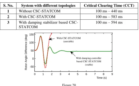
If the large loading duration is increased from 0.1 s to 0.59 s then, the system without damping stabilizer becomes unstable as shown in Figure 20, but the damping stabilizer based CSC-STATCOM still maintains the power system stability. The CCT for the system with & without CSC-STATCOM (and/or damping stabilizer) are shown in Table II. It clearly shows that CCT for the test system is better due to the impact of pole-shifting controller based CSC- STATCOM with damping stabilizer. Hence, the performance of the proposed scheme is satisfactory in this case also.

Table II

CCT of disturbances for the system stability with different topologies (Case-II)

S. No. System with different topologies Critical Clearing Time (CCT)

1 Without CSC-STATCOM 100 ms – 440 ms

2 With CSC-STATCOM 100 ms – 583 ms

3 With damping stabilizer based CSC- STATCOM

100 ms – 594 ms

0 1 2 3 4 5 6 7 8 9

-50 0 50 100 150

Rotor Angle Difference (deg)

Time (s) With CSC-STATCOM

(unstable)

With damping controller based CSC-STATCOM

(stable)

Figure 20

Variation of rotor angle difference of machines M1 & M2 in Case-II (large loading for 0.1 s to 0.59 s)

Conclusions

In this paper, the dynamic modeling of a CSC based STATCOM is studied and pole-shifting controller with damping stabilizer for the best input-output response of CSC-STATCOM is presented in order to enhance the system stability of the power system with the different disturbances. The novelty in proposed approach lies in the fact that, transient stability and oscillation damping ability of a two-area two-machine power system are improved and the critical clearing time of the disturbance is also increased. The coordination between damping stabilizer and pole-shifting controller-based CSC-STATCOM is also shown in the proposed topology. The proposed scheme is simulated and verified with MATLAB software. This paper also shows that a damping stabilizer based CSC-STATCOM is more reliable and effective than a system without damping stabilizer-based CSC-STATCOM, in terms of oscillation damping, critical fault clearing time and transient stability of a two-area power system. Hence, CSC based STATCOM can be regarded as an alternative FACTS device to that of other shunt FACTS devices.

Appendix 1

Parameters for various components used in the test system configuration of Figure 6. (All parameters are in pu unless specified otherwise):

For generator of plant (P1 & P2):

VG=13.8 kV; Rs= 0.003; f=50 Hz; Xd= 1.305; Xd'

= 0.296; Xd''

= 0.252; Xq'

= 0.50; Xq''

= 0.243; Td'

=1.01 s; Td''

=0.053 s; H=3.7 s

(Where Rs is stator winding resistance of generators; VG is generator voltage (L-L), f is frequency; X_d is synchronous reactance of generators; X_d^' & X_d^'' are the transient and sub- transient reactance of generators in the direct-axis; Xq'

& Xq''

are the transient and sub- transient reactance of generators in the quadrature-axis; T_d^' & T_d^'' are the transient and sub- transient open-circuit time constant; H the inertia constant of machine.)

For excitation system of machines (M1 & M2):

Regulator gain and time constant (Ka & Ta): 200, 0.001 s; Gain and time constant of exciter (Ke & Te): 1, 0 s; Damping filter gain and time constant (Kf & Tf): 0.001, 0.1 s;

Upper and lower limit of the regulator output: 0, 7.

For pole-shifting controller based CSC-STATCOM:

System nominal voltage (L-L): 500 kV; Rdc= 0.01; L_dc=40 mH; C = 400 F;R=0.3 ; L = 2 mH; ω=314; Vb(ref )= 1.

For damping stabilizer:

K_s = 25; T_w = 10; T₁ = 0.050; T₂ = 0.020; T₃ = 3; T₄ = 5.4; V_{s (max)} = 0.35; V_{s (min)} = -0.35 References

[1] Prabha Kundur, “Power System Stability and Control”, McGraw-Hill, 1994 [2] G. Rogers, Power System Oscillations, 344 p, Kluwer Power Electronics &

Power System Series, Springer 2000

[3] A. Tahri, H. M. Boulouiha, A. Allali, T. Fatima, “A Multi-Variable LQG Controller-based Robust Control Strategy Applied to an Advanced Static VAR Compensator”, Acta Polytechnica Hungarica, Vol. 10, No. 4, 2013, pp. 229-247

[4] H. Tsai, C. Chu and S. Lee, "Passivity-based Nonlinear STATCOM Controller Design for Improving Transient Stability of Power Systems", Proc. of IEEE/PES Transmission and Distribution Conference &

Exhibition: Asia and Pacific Dalian, China, 2005

[5] M. H. Haque "Improvement of First Swing Stability Limit by Utilizing Full Benefit of Shunt Facts Devices", IEEE Trans. Power Syst., Vol. 19, No. 4, pp. 1894-1902, 2004

[6] P. Kundur, M. Klein, G. J. Rogers, M. S. Zywno, "Application of Power System Stabilizers for Enhancement of Overall System Stability," IEEE Transactions on Power Apparatus and Systems, Vol. 4, No. 2, pp. 614-626, May 1989

[7] M. A. Abido, “Analysis and Assessment of STATCOM-based Damping Stabilizers for Power System Stability Enhancement”, Electric Power Systems Research, Volume 73, Issue 2, pp. 177-185, February 2005 [8] M. Aliakbar Golkar and M. Zarringhalami, “Coordinated Design of PSS

and STATCOM Parameters for Power System Stability Improvement Using Genetic Algorithm”, Iranian Journal of Electrical and Computer Engineering, Vol. 8, No. 2, Summer-Fall 2009

[9] M. Mahdavian, G. Shahgholian, "State Space Analysis of Power System Stability Enhancement with Used the STATCOM", IEEE/ECTI-CON, pp.

1201-1205, Chiang Mai, Thailand, May 2010

[10] N. Mithulananthan, C. A Canizares, J. Reeve and G. J. Rogers,

"Comparison of PSS, SVC and STATCOM Controllers for Damping Power System Oscillations", IEEE Transactions on Power Systems, Vol. 18, No.

2, pp. 786-792, May 2003

[11] Y. L Abdel-Magid & M. A Abido, "Coordinated Design of a PSS & a SVC-based Controller to Enhance Power System Stability", Electrical Power & Energy System, Vol. 25, pp. 695-704, 2003

[12] N. C. Sahoo, B. K. Panigrahi, P. K. Dash and G. Panda, “Multivariable Nonlinear Control of STATCOM for Synchronous Generator Stabilization”, International Journal of Electrical Power & Energy Systems, Volume 26, Issue 1, pp. 37-48, January 2004

[13] L. J. Cai and I. Erlich "Simultaneous Coordinated Tuning of PSS and FACTS Damping Controllers in Large Power Systems", IEEE Trans.

Power Syst., Vol. 20, No. 1, pp. 294-300, 2005

[14] N. G. Hingorani and L. Gyugyi, Understanding FACTS: Concepts and Technology of Flexible ac Transmission Systems, IEEE Press, New York, 1999

[15] Bilgin, H. F., Ermis M., Kose, et al, "Reactive-Power Compensation of Coal Mining Excavators by Using a New-Generation STATCOM ", IEEE Transactions on Industry Applications, Vol. 43, No. 1, pp. 97-110, Jan.-feb.

2007

[16] M. Kazearni and Y. Ye, "Comparative Evaluation of Three-Phase PWM Voltage- and Current-Source Converter Topologies in FACTS Applications", Proc. IEEE Power Eng. Soc. Summer Meeting, Vol. 1, p.

473, 2002

[17] D. Shen and P. W. Lehn, "Modeling, Analysis, and Control of a Current Source Inverter-based STATCOM", IEEE Transactions Power Delivery, Vol. 17, p. 248, 2002

[18] Sandeep Gupta and R. K. Tripathi, “An LQR and Pole Placement Controller for CSC-based STATCOM," in Proc. Inter. Conf. IEEE Power, Energy and Control (ICPEC), pp. 115-119, 2013

[19] C. Schauder and H. Mehta "Vector Analysis and Control of Advanced Static VAR Compensators", IEE Proceedings of Generation, Transmission and Distribution, Vol. 140, pp. 299, 1993

[20] Katsuhiko Ogata, "Modern Control Engineering", 5^th Edition, Prentice Hall, 2010

[21] K. R. Padiyar, V. Swayam Prakash, “Tuning and Performance Evaluation of Damping Controller for a STATCOM”, International Journal of Electrical Power & Energy Systems, Vol. 25, Issue 2, pp. 155-166, February 2003

[22] Ahmad Rohani, M. Reza Safari Tirtashi, and Reza Noroozian, “Combined Design of PSS and STATCOM Controllers for Power System Stability Enhancement”, Journal of Power Electronics, Vol. 11, No. 5, September 2011

[23] B. T. Ooi, M. Kazerani, R. Marceau, Z. Wolanski, F. D. Galiana, D.

McGillis and G. Joos "Mid-Point Sitting of Facts Devices in Transmission Lines", IEEE Trans. Power Del., Vol. 12, No. 4, pp. 1717-1722, 1997