Robust stability of milling operations based on pseudospectral approach
David Hajdu
a,b,∗, Francesco Borgioli
c, Wim Michiels
c, Tamas Insperger
a,dand Gabor Stepan
a,eaDepartment of Applied Mechanics, Budapest University of Technology and Economics, H-1111 Budapest, Hungary
bMTA-BME Lendület Machine Tool Vibration Research Group, H-1111 Budapest, Hungary
cDepartment of Computer Science, KU Leuven, Celestijnenlaan 200A, Leuven 3001, Belgium
dMTA-BME Lendület Human Balancing Research Group, H-1111 Budapest, Hungary
eMTA-BME Research Group on Dynamics of Machines and Vehicles, H-1111 Budapest, Hungary
A R T I C L E I N F O
Keywords: Chatter Collocation
Pseudospectral method Robustness
Uncertainty
A B S T R A C T
The prediction of chatter-free machining parameters is not reliable for industrial applications without guaranteed robustness against modeling uncertainties. Measurement inaccuracies, fitting uncertain- ties, simplifications and modeling errors typically lead to a mismatch between the mathematical model and the real physical system. This paper presents the robust stability analysis of milling operations based on a pseudospectral approach to take into account the effect of bounded parametric uncertainties both in the cutting coefficients and in the modal parameters. In order to make the predictions more accurate, the operational modal analysis of the spindle during rotation was conducted. The natural fre- quencies and damping ratios of the dominant vibration modes were identified from the impact tests of the rotating tool at different spindle speeds. The uncertainties of the fitted parameters were included in the computation of the pseudospectral radius of the monodromy operator of the time-periodic system.
The solver is tested in a case study and experimental chatter tests are also included for demonstration purposes.
Digital Object Identifier:10.1016/j.ijmachtools.2019.103516
1. Introduction
The continuously increasing demand for competitive, fast, high-quality and economical production forces the manufac- turing industry to push the operational conditions of ma- chines to their limit. However, after a certain point often quality and reliability decreases, while deterioration and costs increase. In material removal processes, such as milling, turning, grinding, or drilling, one of the most destructive phenomenon that limits productivity the most is machine tool vibration [1].
The first mathematical equations describing the evolu- tion of unstable vibrations appeared in the work of Tobias [2]
and Tlusty [3] in the 1950s and 1960s, although the impor- tance of the phenomenon was already recognized by Taylor at the beginning of the 20th century [4]. Their observations laid down the fundamentals of the so-called surface regener- ation effect, which became the most widely accepted expla- nation for machine tool vibration. The geometry of the chip is modified by the relative motion between the tool and work- piece, which induces variation in the cutting force. The vi- brations in the past are embedded in the surface of the work- piece, which affects every subsequent cut by the modified geometry of the chip that depends on present and past states, too. Dependencies on past events in dynamical models are described by delay-differential equations (DDEs). When the stationary solution of the DDE loses stability, the amplitude of vibration increases until the physical contact between the workpiece and the tool is lost. This large-amplitude self- excited vibration is called chatter.
∗Corresponding author hajdu@mm.bme.hu(D. Hajdu)
A milling operation is an intermittent cutting process, where the chip geometry varies periodically at every tooth- passing interval. The surface regeneration couples with para- metric excitation and results in a DDE with periodically vary- ing coefficients, also called time-periodic delay-differential equation (TPDDE). The stationary solution in a stable opera- tion is periodic (at most with the spindle revolution period), which can undergo secondary Hopf or period doubling bi- furcations [5] as the machining parameters change.
The harmful unstable vibrations must be avoided during the operation in order to reach the required quality and max- imize the production. The highest performance of machin- ing centers, however, can only be reached if the machine is safely operated at high speeds close to stability boundaries.
These conditions require a reliable and accurate prediction of dynamical behavior. The domain of chatter-free machining parameters are visualized by the so-called stability lobe dia- grams. Nevertheless, deterministic models considered dur- ing calculations often fail to accurately predict dynamical behavior and therefore experimental cutting tests do not al- ways match the expectations. One of the reason is the uncer- tainties in the dynamical model that affect the prediction of chatter-free machining parameters.
The need for reliable predictions considering variations in machining and dynamical parameters was already rec- ognized by the engineering community, and many attempts were made to construct such stability lobe diagrams that take the effect of modeling errors into account. These diagrams are referred to as robust stability lobe diagrams, where the domain of robust stable machining parameters can retain the stability if bounded uncertainties in the model arise. In the simplest case, Monte Carlo simulations and statistical eval- uations were performed in [6,7], which require significant computational effort and therefore their practical applica-
tion without major improvements is limited. The advan- tage of these methods, however, is the statistical data pro- vided after a large amount of computations. To obtain sim- ilar results without huge computational efforts, research pa- pers also provide local sensitivity methods, e.g. [8,9,10], that are based on local derivatives (sensitivity) and extrap- olations. A global sensitivity method is presented in [11], which approximates a multi-dimensional integral of the prob- ability density function (PDF) by separated one-dimensional integrals. The Robust Chatter Prediction Method (RCPM) presented in [12] is also an alternative method for global analysis, which is based on the discretization of the PDF.
Robust methods, where the worst-case perturbations are sought, were also used in the literature. For instance, the Edge Theorem combined with the Zero Exclusion Princi- ple presented in [13] provides robust stability boundaries for time-invariant models, but the computational effort is often large. A different robust method called Multi-frequency So- lution with Structured Singular Value Analysis is based on the direct perturbation of the measured frequency response functions (FRFs), where parameter perturbations are replaced by FRF perturbations, see [14]. In this latter case the com- putational effort is significantly reduced, but the prediction can be very conservative.
This paper presents the application of a pseudospectral approach that considers uncertainties in the dynamical pa- rameters of milling operations and provides robust stable machining domains to exploit the highest productivity. The method is based on an iterative solver, that computes the worst-case uncertainty and therefore no conservativeness is introduced. In order to make the computations effective, the calculation of the characteristic multipliers (Floquet multi- pliers) of the time-periodic DDE is carried out by discretiz- ing the eigenvalue problem of the monodromy operator into a generalized eigenvalue problem (GEP), using a spectral method. The iterations converge to a local maximizer of the pseudospectral radius in the space of allowable pertur- bations. However, global optimality is achieved by incor- porating a restarting strategy, where several dominant Flo- quet multipliers of the original system are used to initialize the iteration. The related problem of computing the globally rightmost point of pseudospectra of time-invariant systems is addressed in [15].
The paper is structured as follows. In Sec.2the dynami- cal model of milling operations is presented, then the stabil- ity of time-periodic DDEs is investigated in Sec.3by intro- ducing the new formalism. The pseudospectral approach to access robust stability is detailed in Sec.4. A case study to test the computation of robust boundaries along with exper- imental chatter tests are presented in Sec.5. The calculated stability boundaries are compared to a structured singular value analysis in Sec.6. The conclusions are presented in Sec.7.
2. Modeling of milling operations
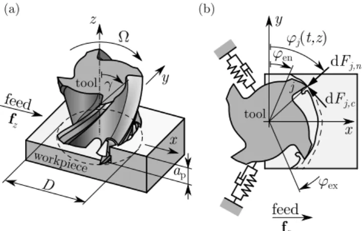
A regular cutting tool with uniform helix angle is pre- sented in Fig.1(a). The equation of motion of the tool-tip
z
x y feed
workpiece tool
ap
j(t,z)
en
D ex
x
(a) (b) y
fz
feed fz
tool
dFj,n dFj,c
j
Figure 1:Dynamical model of milling in case of regular cutting tools with diameter 𝐷, helix angle𝛾 = 45◦, 𝑍𝑡 = 4 cutting edges and depth of cut𝑎p. (a) Three-dimensional model; (b) Cutting forces acting on an elementary disk of widthd𝑧.
subjected to time-dependent forcing can be described in the modal space by introducing the vector of the modal coordi- nates𝐪(𝑡) ∈ ℝ𝑑. In case of proportional damping models, the eigenmodes of the system are real and the equation can be transformed into the form
𝐪(𝑡)+[2𝜁̈ 𝑙𝜔n,𝑙]𝐪(𝑡)+[𝜔̇ 2n,𝑙]𝐪(𝑡) =𝐔⊤𝐅(
𝑡,𝐫(𝑡),𝐫(𝑡−𝜏)) , (1) where 𝐅(𝑡,⋅) ∈ ℝ2 is the forcing vector at the tool-tip in the (𝑥,𝑦)-plane,𝑑is the modeled number of degrees of free- dom,[⋅] = diag(⋅) ∈ℝ𝑑×𝑑are diagonal matrices,𝜔n,𝑙is the 𝑙-th natural angular frequency (𝑙 = 1,…, 𝑑),𝜁𝑙 is the cor- responding relative damping ratio,𝐫(𝑡) = [𝑥(𝑡), 𝑦(𝑡)]⊤ de- notes the displacement of the tool-tip in the (𝑥,𝑦)-plane and 𝐔∈ℝ2×𝑑is the modal transformation matrix that connects the modal space and the tool-tip’s motion as𝐫(𝑡) = 𝐔𝐪(𝑡) [16].
The cutting force acting at the tool-tip is described by empirical force models, that highly depend on the tool ge- ometry and material properties. Next, for sake of brevity, regular cutting tools with𝑍𝑡number of equally distributed cutting edges and with uniform helix angle𝛾 are modeled.
Thus, the angular position of the𝑗-th cutting edge (𝑗= 1,…, 𝑍𝑡) along the axial direction reads
𝜑𝑗(𝑡, 𝑧) = Ω2𝜋 60𝑡+2𝜋
𝑍𝑡𝑗−2 tan𝛾
𝐷 𝑧, (2)
where 𝑧 is the coordinate along the axial immersion and Ωis the spindle speed given in rpm. The cross-section of the cutter is presented in Fig.1(b). The elementary cutting- force components in tangential and radial directions acting on tooth𝑗at a disk element of width d𝑧are given as
d𝐹𝑗,𝑐(𝑡, 𝑧) =𝑔𝑗(𝑡, 𝑧)𝐾𝑐ℎ( ℎ𝑗(𝑡, 𝑧))
d𝑧, (3)
d𝐹𝑗,𝑛(𝑡, 𝑧) =𝑔𝑗(𝑡, 𝑧)𝐾𝑛ℎ( ℎ𝑗(𝑡, 𝑧))
d𝑧, (4)
whereℎ𝑗(𝑡, 𝑧)is the theoretical chip thickness cut by tooth 𝑗at axial immersion𝑧, moreover𝐾𝑐ℎ(ℎ)and𝐾𝑛ℎ(ℎ)are the
empirical cutting force characteristics assumed in the shifted linear form
𝐾𝑐ℎ(ℎ) =𝑘𝑐𝑝+𝑘𝑐𝑠ℎ,
𝐾𝑛ℎ(ℎ) =𝑘𝑛𝑝+𝑘𝑛𝑠ℎ, (5)
where 𝑘𝑐𝑝 and𝑘𝑐𝑠 are cutting coefficients in the main di- rection (tangential), and𝑘𝑛𝑝and𝑘𝑛𝑠are cutting coefficients in radial direction according to the Shearing & Ploughing (S&P) cutting force model [17]. The indicator function𝑔𝑗(𝑡, 𝑧) is a piecewise constant function, which gives whether the cutting edge is in contact with the material or not. 𝑔𝑗(𝑡)can be written as
𝑔𝑗(𝑡, 𝑧) = {
1, if𝜑en<(
𝜑𝑗(𝑡, 𝑧)mod2𝜋)
< 𝜑ex,
0, otherwise, (6)
where𝜑enis the angle where the elementary disk starts cut- ting and𝜑exis the angular position where it leaves the work- piece, see Fig.1(b). The actual chip thickness cut by tooth 𝑗at axial immersion𝑧then can be calculated approximately as
ℎ𝑗(𝑡, 𝑧) ≈
[sin𝜑𝑗(𝑡, 𝑧) cos𝜑𝑗(𝑡, 𝑧)
]⊤(
𝐟𝑧+𝐫(𝑡) −𝐫(𝑡−𝜏)) , (7) where𝐟𝑧 = [𝑓𝑧,0]⊤is the feed per tooth in direction𝑥, and the time-delay (equal to the tooth-passing period) in case of equally distributed cutting edges is𝜏 = 60∕(𝑍𝑡Ω). The re- sultant cutting force vector in the (𝑥,𝑦)-plane concentrated theoretically at the tool-tip is calculated as
𝐅(𝑡,⋅) = −
𝑍𝑡
∑
𝑗=1∫
𝑎p 0
𝐓𝑗(𝑡, 𝑧) [𝐾𝑐ℎ(
ℎ𝑗(𝑡, 𝑧)) 𝐾𝑛ℎ(
ℎ𝑗(𝑡, 𝑧))]
𝑔𝑗(𝑡, 𝑧)d𝑧, (8) where the transformation matrix is written as
𝐓𝑗(𝑡, 𝑧) =
[cos𝜑𝑗(𝑡, 𝑧) sin𝜑𝑗(𝑡, 𝑧)
− sin𝜑𝑗(𝑡, 𝑧) cos𝜑𝑗(𝑡, 𝑧) ]
. (9)
Inserting the regenerative forcing model into the govern- ing equation, then assuming small perturbation𝜺(𝑡)about the periodic motion𝐪p(𝑡)of the stationary cutting, i.e.,𝐪(𝑡) = 𝐪p(𝑡) +𝜺(𝑡), the equation of the variational system omitting the periodic term is written as
𝜺(𝑡)+[2𝜁̈ 𝑙𝜔n,𝑙]𝜺(𝑡)+[𝜔̇ 2n,𝑙]𝜺(𝑡) =𝐔⊤𝐐(𝑡)𝐔(
𝜺(𝑡)−𝜺(𝑡−𝜏)) , (10) where the directional matrix𝐐(𝑡) = 𝐐(𝑡+𝜏)is introduced as
𝐐(𝑡) = 𝜕𝐅
𝜕𝐫(𝑡)
(𝑡,𝐫p(𝑡),𝐫p(𝑡−𝜏))
=
= −
𝑍𝑡
∑
𝑗=1∫
𝑎p 0
𝐓𝑗(𝑡, 𝑧) [𝑘𝑐𝑠
𝑘𝑛𝑠
] (sin𝜑𝑗(𝑡, 𝑧) cos𝜑𝑗(𝑡, 𝑧)
)⊤
𝑔𝑗(𝑡, 𝑧)d𝑧, (11)
where the dependency on𝑔𝑗(𝑡, 𝑧) for𝑗 = 1,…, 𝑍𝑡 make 𝐐(𝑡) discontinuous, but piecewise smooth, see [18]. The time-periodic DDE (10) can be rewritten into a first-order form [
𝜺(𝑡)̇ 𝜺(𝑡)̈ ]
=
[ 𝟎𝑑 𝐈𝑑
−[𝜔2n,𝑙] +𝐔⊤𝐐(𝑡)𝐔 −[2𝜁𝑙𝜔n,𝑙] ] [𝜺(𝑡)
𝜺(𝑡)̇ ]
+ [ 𝟎𝑑 𝟎𝑑
−𝐔⊤𝐐(𝑡)𝐔 𝟎𝑑
] [𝜺(𝑡−𝜏) 𝜺(𝑡̇ −𝜏) ]
. (12)
where𝐈𝑑is the𝑑×𝑑identity matrix and𝟎𝑑is the𝑑×𝑑zero matrix.
3. Stability of time-periodic time-delay systems
We observe that the governing equation (12) is of the form
𝐱(𝑡) =̇ 𝐀(𝑡)𝐱(𝑡) +𝐁(𝑡)𝐱(𝑡−𝜏), (13) where𝐱(𝑡) ∈ ℝ𝑛 is the vector of state variables at time𝑡, and𝐀,𝐁areℝ𝑛×𝑛-valued periodic functions with main pe- riod𝑇 = 𝜏. In the present and in the following section we briefly illustrate a novel pseudospectral approach to assess the stability robustness of a system of time-periodic DDEs, which was introduced in a more general form in [19]. In this manuscript we adapt the description to systems of the form (13). We first explain the adopted approach for gen- eral matrix-valued functions𝐀and𝐁. At the end of the sec- tion, we explain how the method can be improved by exploit- ing the property that the coefficients in (12) are piecewise smooth functions.
The solution of the infinite-dimensional time-delay sys- tem governed by (13) depends on the time history of𝐱(𝑡), therefore an initial function is required to determine the evo- lution of states in time. In order to generalize the notation, let=([−𝜏,0],ℂ𝑛)be the space of continuous functions on the interval𝐼 = [−𝜏,0]and let us introduce the notation 𝐱𝑡 ∶= 𝐱(𝑡+𝜗),𝜗 ∈ [−𝜏,0]in order to denote the solution segment over the interval[𝑡−𝜏, 𝑡]. The Cauchy problem associated with the system (13) is written as
{𝐱(𝑡) =̇ 𝐀(𝑡)𝐱(𝑡) +𝐁(𝑡)𝐱(𝑡−𝜏), 𝑡 > 𝑡0, 𝐱(𝑡0+𝜗) =𝐱𝑡
0, 𝜗∈ [−𝜏,0], (14)
with𝐱𝑡
0 ∈being the initial function. The solution segment of the system at any time𝑡associated with the initial function 𝐱𝑡
0 is described by the evolution operator(𝑡, 𝑡0) ∶→, defined through the relation
𝐱𝑡=(𝑡, 𝑡0)𝐱𝑡
0. (15)
The asymptotic stability of the trivial solution𝐱(𝑡) ≡𝟎 of (13) is determined by the spectral properties of the mon- odromy operator ∶= (𝑇 ,0) (setting𝑡0 = 0), as it is proven by the Floquet theory [20]. The nonzero elements of the spectrum ofare called characteristic multipliers (or Floquet multipliers) and can also be defined by
Ker(𝜇−)≠{𝟎}, 𝜇≠0, (16)
withbeing the identity operator. Any𝜇 ∈ ℂ,𝜇 ≠0is a Floquet multiplier if and only if there exists an eigenfunction 𝝋∈,𝝋≠𝟎, such that
(𝑡+𝑇 ,0)𝝋=𝜇(𝑡,0)𝝋, for all𝑡≥0. (17) In general, there are no explicit expressions for the evo- lution operator and the characteristic multipliers. However, several numerical methods exist for approximating the oper- ator and the multipliers.
As examples, interested readers are referred to numeri- cal methods such as the Semidiscretization technique [5], the Spectral Element Method [21], [22], Chebyshev polynomial- based collocation methods [23,24] or the Improved Cheby- shev Collocation Method [17], just to mention a few. In or- der to provide a technique amendable for the adopted pseudospectra- based approach towards uncertainty, a different Chebyshev polynomial-based approach is presented: as we will see, the Floquet multipliers are computed as the eigenvalues of a gen- eralized eigenvalue problem which preserves linearity w.r.t.
the entries of the nominal matrices𝐀and𝐁.
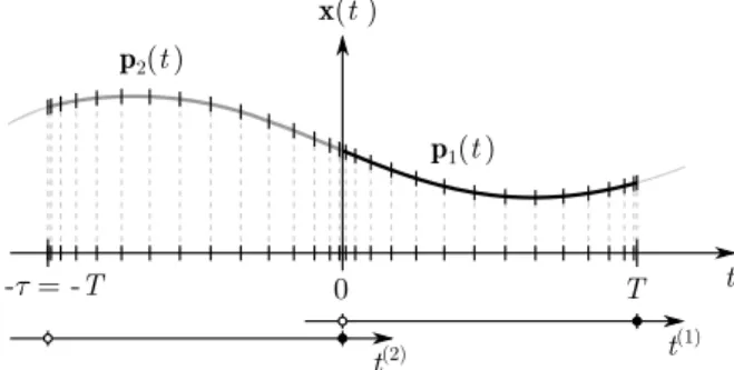
For systems like (13), where 𝑇 = 𝜏, the proposed ap- proach approximates the solution𝐱on the interval[−𝜏, 𝑇] by a piecewise polynomial𝐩in the form
𝐱(𝑡) ≈𝐩(𝑡) =
∑2
𝑗=1
𝐩𝑗(𝑡)𝐼𝑗(𝑡), (18) where𝐼𝑗(𝑡)is the indicator function of the interval 𝐼𝑗 (1 if𝑡 ∈ 𝐼𝑗, and0otherwise), and where𝐼2 = [−𝜏,0],𝐼1 = [0, 𝑇], as it is seen in Fig.2. We consider the mesh{𝛼𝑙}𝑀+1𝑙=1 of Chebyshev-distributed points on the interval[−1,1]
𝛼𝑙= − cos ( 𝜋𝑙
𝑀+ 1 )
, 𝑙= 1,…, 𝑀+ 1, (19) 𝑀+ 1is the number of Chebyshev-distributed points, from which we can define the mesh{𝑡(𝑗)𝑙 }𝑀+1𝑙=1 on any𝐼𝑗 = [𝑎𝑗, 𝑏𝑗] (and viceversa) by using the following transformations
𝑡(𝑗)𝑙 ∶=1 2
(𝑎𝑗+𝑏𝑗) +𝛼𝑙
2
(𝑏𝑗−𝑎𝑗)
, 𝑡(𝑗)𝑙 ∈𝐼𝑗, 𝛼𝑙=𝑤𝑗(
𝑡(𝑗)
𝑙
)= (
𝑡(𝑗)
𝑙 −1 2
(𝑎𝑗+𝑏𝑗)) 2
𝑏𝑗−𝑎𝑗. (20) The solution is approximated on each interval based on a linear combination of Chebyshev polynomials (𝑇𝑠) of the first kind with degree𝑠as
𝐩𝑗(𝑡) =
∑𝑀
𝑠=0
𝐜(𝑗)𝑠 𝑇𝑠( 𝑤𝑗(𝑡))
, (21)
and𝐜(𝑗)𝑠 ∈ℂ𝑛are the coefficients to be determined. In order to formulate the solution in terms of the polynomials, the following conditions are imposed:
• Collocation constraint for (17) for𝑙= 1,…, 𝑀+ 1 𝜇
∑𝑀
𝑠=0
𝐜(2)𝑠 𝑇𝑠(𝛼𝑙) −
∑𝑀
𝑠=0
𝐜(1)𝑠 𝑇𝑠(𝛼𝑙) =𝟎. (22)
t x(t )
p2(t)
0 T - = -T
t t
p1(t)
Figure 2: Discretization of 𝐱(𝑡) at the Chebyshev points over the domain[−𝜏, 𝑇].
• Continuity in𝑡= 0gives𝐩2(0) =𝐩1(0), i.e.,
−
∑𝑀
𝑠=0
𝐜(1)𝑠 𝑇𝑠(−1) +
∑𝑀
𝑠=0
𝐜(2)𝑠 𝑇𝑠(1) =𝟎. (23)
• Collocation constraint for the TPDDE (13) gives 𝐩(𝑡̇ (1)𝑙 ) =𝐀(𝑡(1)𝑙 )𝐩(𝑡(1)𝑙 ) +𝐁(𝑡(1)𝑙 )𝐩(𝑡(1)𝑙 −𝜏), (24) for𝑙= 1,…, 𝑀+ 1,which using (21) gives
∑𝑀
𝑠=1
𝐜(1)𝑠 2
𝑇𝑠𝑈𝑠−1(𝑤1(𝑡(1)𝑙 )) −
∑𝑀
𝑠=0
𝐀(𝑡(1)𝑙 )𝐜(1)𝑠 𝑇𝑠(𝑤1(𝑡(1)𝑙 ))+
−
∑𝑀
𝑠=0
𝐁(𝑡(1)𝑙 )𝐜(2)𝑠 𝑇𝑠(𝑤2(𝑡(2)𝑙 )) =
∑𝑀
𝑠=1
𝐜(1)𝑠 2
𝑇𝑠𝑈𝑠−1(𝛼𝑙) −
∑𝑀
𝑠=0
𝐀(𝑡(1)𝑙 )𝐜(1)𝑠 𝑇𝑠(𝛼𝑙)+
−
∑𝑀
𝑠=0
𝐁(𝑡(1)𝑙 )𝐜(2)𝑠 𝑇𝑠(𝛼𝑙) =𝟎 (25) for all𝑙 = 1,…, 𝑀. Here, we have applied the fact that𝑤′(𝑡(1)𝑙 ) = 2∕𝑇and𝑇̇𝑠(𝑡) =𝑠𝑈𝑠−1(𝑡), where𝑈𝑠(𝑡) is the Chebyshev polynomial of the second kind of de- gree𝑠.
The conditions above result a generalized eigenvalue prob- lem in the form
(𝐒−𝐑𝜇)𝐂=𝟎, (26)
where 𝐂 = [𝐜(2)0 ,…,𝐜(2)
𝑀,𝐜(1)
0 ,…,𝐜(1)
𝑀]⊤ ∈ ℂ2𝑛(𝑀+1) and 𝐑,𝐒 ∈ ℝ2𝑛(𝑀+1)×2𝑛(𝑀+1). The coefficient matrices in (26) can be expressed as follows
𝐑=
[𝐑11 𝟎 𝟎 𝟎 ]
, 𝐒=
[ 𝟎 𝐒12 𝐒21 𝐒22 ]
, (27)
where
𝐑11=𝐒12=
⎡⎢
⎢⎣
𝑇0(𝛼1)𝐈𝑛 ⋯ 𝑇𝑀(𝛼1)𝐈𝑛
⋮ ⋱ ⋮
𝑇0(𝛼𝑀+1)𝐈𝑛 ⋯ 𝑇𝑀(𝛼𝑀+1)𝐈𝑛
⎤⎥
⎥⎦ , (28)
𝐒21= −
⎡⎢
⎢⎢
⎢⎣
𝐁(𝑡(1)1 )𝑇0(𝛼1)𝐈𝑛 ⋯ 𝐁(𝑡(1)1 )𝑇𝑀(𝛼1)𝐈𝑛
⋮ ⋱ ⋮
𝐁(𝑡(1)𝑀)𝑇0(𝛼𝑀)𝐈𝑛 ⋯ 𝐁(𝑡(1)𝑀)𝑇𝑀(𝛼𝑀)𝐈𝑛 𝑇0(1)𝐈𝑛 ⋯ 𝑇𝑀(1)𝐈𝑛
⎤⎥
⎥⎥
⎥⎦ , (29)
𝐒22=
⎡⎢
⎢⎢
⎢⎣ 𝟎𝑛 2
𝑇𝑈0(𝛼1)𝐈𝑛 ⋯ 𝑀2
𝑇𝑈𝑀−1(𝛼1)𝐈𝑛
⋮ ⋮ ⋱ ⋮
𝟎𝑛 2
𝑇𝑈0(𝛼𝑀)𝐈𝑛 ⋯ 𝑀2
𝑇𝑈𝑀−1(𝛼𝑀)𝐈𝑛
𝟎𝑛 𝟎𝑛 ⋯ 𝟎𝑛
⎤⎥
⎥⎥
⎥⎦
−
⎡⎢
⎢⎢
⎢⎣
𝐀(𝑡(1)1 )𝑇0(𝛼1)𝐈𝑛 ⋯ 𝐀(𝑡(1)1 )𝑇𝑀(𝛼1)𝐈𝑛
⋮ ⋱ ⋮
𝐀(𝑡(1)𝑀)𝑇0(𝛼𝑀)𝐈𝑛 ⋯ 𝐀(𝑡(1)𝑀)𝑇𝑀(𝛼𝑀)𝐈𝑛
−𝑇0(−1)𝐈𝑛 ⋯ −𝑇𝑀(−1)𝐈𝑛
⎤⎥
⎥⎥
⎥⎦ ,
(30)
When𝐀and𝐁are smooth functions, the solutions emanat- ing from an eigenfunction are smooth on[−𝜏,0]and[0, 𝑇];
hence, they can be well approximated by polynomials on each of these intervals, ensuring spectral convergence of the eigenvalue approximations as a function of the degree𝑀. However, if𝐀and𝐁are only piecewise smooth, as might be the case for (12), the discontinuities in𝐀and𝐁impact the smoothness of the solutions and negatively affect the con- vergence rate of polynomial approximations. However, this problem can be overcome by a choice of piecewise polyno- mial consistent with the location of the discontinuities, while at the intersections only continuity is imposed. We refer the reader interested in a more detailed description on interval splitting to [19,22] or [24].
4. Pseudospectral method for robust analysis
In this section we assume that the generic system of time- periodic DDEs (13) is affected by a set of real-valued scalar uncertainties, that result the perturbed equation in the form
𝐱(𝑡) =̇ (
𝐀(𝑡) +
∑𝐾
𝑘=1
𝐃0𝑘(𝑡)Δ𝑘𝐄⊤0𝑘(𝑡) )
𝐱(𝑡)+
( 𝐁(𝑡) +
∑𝐾
𝑘=1
𝐃1𝑘(𝑡)Δ𝑘𝐄⊤1𝑘(𝑡) )
𝐱(𝑡−𝜏), (31) where Δ𝑘 ∈ ℝ, 𝑘 = 1,…, 𝐾,are the uncertainties, and 𝐃𝑖𝑘(𝑡), 𝐄𝑖𝑘(𝑡) ∈ ℝ𝑛 (𝑖 = 0,1, 𝑘 = 1,…, 𝐾) are time- periodic scaling matrices defining the structure and the weight of each uncertaintyΔ𝑘(this will be clarified in the numerical experiments). We indicate each vector of uncertainties with the compact notation𝚫 = [Δ1,…,Δ𝐾]⊤ ∈ ℝ𝐾. In addi- tion, we set an upper bound equal to1on the absolute value of eachΔ𝑘, i.e.,|Δ𝑘| ≤ 1 for𝑘 = 1,…, 𝐾: observe that this can be done without loosing of generality, since we can assign different weights to each uncertainty using the scal- ing matrix-valued functions𝐃𝑖𝑘,𝐄𝑖𝑘. For the more complex case of matrix-valued uncertainties𝚫𝑘 we refer again the reader to [19].
Each uncertaintyΔ𝑘perturbing the time-periodic matrix 𝐀or𝐁necessarily affects the collocation constraints for the TPDDE defined in (25) for𝑙 = 1,…, 𝑀 + 1: thus we re- define the generalized eigenvalue problem corresponding to (26) as
𝐹(𝜇;𝚫)𝐂∶=((
𝐒+
∑𝐾
𝑘=1
𝛿𝐒(𝑘))
−𝐑𝜇 )
𝐂=𝟎, (32) where𝛿𝐒(𝑘)indicates the perturbation of𝐒induced by para- metric uncertaintyΔ𝑘. The construction of the perturbation matrix is given in the AppendixA.
In order to analyse the worst-case scenario for this class of perturbations we look for theFloquet pseudospectral ra- dius𝜇𝐿, i.e., the eigenvalue with largest modulus that the perturbed generalized eigenvalue problem (32) can attain.
If the Floquet pseudospectral radius has modulus less than one, then we are guaranteed that the zero solution of (31) is asymptotically stable despite the uncertainties. Hence, the Floquet pseudospectral radius allows to assess the sta- bility robustness. The worst-case analysis is performed by applying a (projected) gradient-ascent method in the space of uncertainties, thereby optimizing the modulus of the dom- inant Floquet multiplier: this approach is conceptually sim- ilar to the state-of-the-art approach ([15,25]) in the worst- case analysis of time-invariant functional-differential equa- tions, where the rightmost eigenvalue generated by a class of bounded perturbations is maximized.
To compute the Floquet pseudospectral radius we solve the optimization problem
max |𝜇𝐷|
s.t. 𝚫∈ℝ𝐾, |Δ𝑘|≤1, for each𝑘= 1,…, 𝐾, (33) where𝜇𝐷is the dominant eigenvalue of perturbed problem
𝐹(𝜇;𝚫)𝐯=𝟎, for some𝐯∈ℂ2𝑛(𝑀+1). (34) This problem can be solved by simply using a projected gra- dient method in the space of1-bounded perturbations𝚫: in the following we first construct the gradient of the dominant eigenvalue𝜇𝐷of the perturbed generalized eigenvalue prob- lem (32) w.r.t. to uncertaintiesΔ𝑘. Let𝐮,𝐯 ∈ℂ2𝑛(𝑀+1)be the left and the right eigenvector of𝜇𝐷with unit norms and such that𝜉∶=𝐮∗𝐑𝐯>0, where𝐮∗is the complex conjugate of𝐮. The derivative of|𝜇𝐷|2w.r.t. Δ𝑘as follows
𝐺𝑘∶= 𝜕|𝜇𝐷|2
𝜕Δ𝑘 = 2ℜ (
𝜇∗𝐷𝜕𝜇𝐷
𝜕Δ𝑘 )
= 2 𝜉ℜ
(
𝜇𝐷∗𝐮∗𝜕𝛿𝐒(𝑘)
𝜕Δ𝑘 𝐯 )
, (35) for𝑘 = 1,…, 𝐾. Note, that𝛿𝐒(𝑘) depends affinely on the uncertaintyΔ𝑘, and therefore𝜕𝛿𝐒(𝑘)∕𝜕Δ𝑘is a (sparse) ma- trix, which does not change during the iterations. Therefore the calculation of𝐺𝑘in (35) is numerically efficient. A fast way to compute𝐺𝑘 is given in AppendixA. We can now use a (projected) gradient method to solve the optimization
problem (33) using the following fundamental step at each iteration𝓁
Δ(𝓁+1)𝑘 = Δ(𝓁)𝑘 +𝛾𝓁𝑃𝑘(𝓁), 𝑘= 1,…, 𝐾, (36) where𝛾𝓁is the stepsize at iteration𝓁and𝑃𝑘(𝓁)is the ascent direction defined as follows
𝑃(𝓁)
𝑘 =
{0, if|Δ(𝓁)𝑘 |= 1, sign(𝐺(𝓁)𝑘 Δ(𝓁)𝑘 )>0, 𝐺𝑘(𝓁), otherwise,
(37) where𝐺(𝓁)
𝑘 is the derivative of thelargest eigenvalueof the generalized eigenvalue problem (32) perturbed with uncer- taintiesΔ(𝓁)𝑘 . Observe that𝑃(𝓁)
𝑘 is the projection of the deriva- tive𝐺(𝓁)
𝑘 on the feasible set, which is needed to avoid the violation of the norm constraint.
4.1. Implementation
We here provide some more technical details about the implementation of the described method: the algorithm is stopped at some iteration𝓁such that the norm of the (pro- jected) derivative 𝑃(𝓁)
𝑘 is below a prescribed tolerance for 𝑘= 1,…, 𝐾; of course, being a gradient ascent method, this algorithm is not guaranteed to converge globally rather than locally. Sticking to the state of the art (see [25,26]), includ- ing the following strategies in order to compute the globally dominant Floquet multiplier has proved to be effective:
• The adaptive stepsize guarantees the monotonicity of the iterations: at each step𝓁, the initial step𝛾𝓁−1is re- duced by a scaling factor 2 until monotonicity is guar- anteed; vice versa, if𝛾𝓁−1already guarantees mono- tonicity, an extra computation with a doubled step- size is carried out: the stepsize𝛾𝓁 that guarantees the largest eigenvalue is then adopted.
• The restarting strategy: the method is run multiple times, each time initializingΔ(0)𝑘 , 𝑘 = 1, ..., 𝐾,from the left and right eigenvectors (see [15] for the details) corresponding to several dominant eigenvalues of the unperturbed problem.
4.2. Extension to modal parameter uncertainties The application of the pseudospectral method relies on a numerically efficient computation of the gradient in (35). In order to apply the strategies discussed in this paper, we need the governing equation (including the perturbations) to be represented in the form of (31). In order to make the method easily applicable to system (12), we introduce a transforma- tion in this subsection.
The modal parametes𝜔n,𝑙 and𝜁𝑙(and their uncertainty) show up nonlinearly in the system (12), however, the latter can be transformed to a linear form by introducing a slack variable𝒗(𝑡) = [𝜔n,𝑙]𝜺(𝑡), and increasing the dimension of
the state vector. Then, the linearity is established and the system reads as follows
∶=𝐋
⏞⏞⏞⏞⏞⏞⏞⏞⏞⏞⏞⏞⏞⏞⏞⏞⏞⏞⏞
⎡⎢
⎢⎣
𝟎𝑑 𝟎𝑑 𝟎𝑑 𝐈𝑑 𝟎𝑑 𝟎𝑑 𝟎𝑑 𝐈𝑑 [2𝜁𝑙]
⎤⎥
⎥⎦
⎡⎢
⎢⎣ 𝜺(𝑡)̇ 𝜺(𝑡)̈ 𝒗(𝑡)̇
⎤⎥
⎥⎦
=
=𝐀(𝑡)
⏞⏞⏞⏞⏞⏞⏞⏞⏞⏞⏞⏞⏞⏞⏞⏞⏞⏞⏞⏞⏞⏞⏞⏞⏞⏞⏞⏞⏞⏞⏞⏞⏞⏞⏞⏞⏞
⎡⎢
⎢⎣
[𝜔n,𝑙] 𝟎𝑑 −𝐈𝑑 𝟎𝑑 𝐈𝑑 𝟎𝑑 𝐔⊤𝐐(𝑡)𝐔 𝟎𝑑 −[𝜔n,𝑙]
⎤⎥
⎥⎦
⎡⎢
⎢⎣ 𝜺(𝑡) 𝜺(𝑡)̇ 𝒗(𝑡)
⎤⎥
⎥⎦ +
⎡⎢
⎢⎣
𝟎𝑑 𝟎𝑑 𝟎𝑑 𝟎𝑑 𝟎𝑑 𝟎𝑑
−𝐔⊤𝐐(𝑡)𝐔 𝟎𝑑 𝟎𝑑
⎤⎥
⎥⎦
⏟⏞⏞⏞⏞⏞⏞⏞⏞⏞⏞⏞⏞⏞⏞⏟⏞⏞⏞⏞⏞⏞⏞⏞⏞⏞⏞⏞⏞⏞⏟
=𝐁(𝑡)
⎡⎢
⎢⎣ 𝜺(𝑡−𝜏) 𝜺(𝑡̇ −𝜏) 𝒗(𝑡−𝜏)
⎤⎥
⎥⎦ .
(38) Observe that the leading matrix𝐋of the system is not the identity matrix anymore, and that it is perturbed by the un- certainty affecting𝜁𝑙: however, the methodology illustrated in Sec.4can be trivially extended to account for uncertain leading matrices as well. Regarding the computation of Flo- quet multipliers as introduced in Sec.3, it is easy to see that 𝐈𝑛in the definition of the first matrix in𝑺22in (30) must be replaced by𝐋(see the left-hand-side of (24), which has to be modified by introducing 𝐋). Also note that this exten- sion requires two pairs of scaling matrices associated with the perturbation of𝜔n,𝑙, but the implementation of the pseu- dospectral method is not affected.
5. Case study and experiment
Experimentally determined stability limits are often dif- ferent from the ones predicted based on a dynamical model.
It is known that natural frequencies and damping ratios mea- sured on the rotating spindle may differ from the ones mea- sured on the idle tool, and this effect can be responsible for variations in the stability lobe diagrams. However, this char- acteristics can be measured prior to the experiments or pre- dicted based on preliminary chatter tests, see [28,29] and es- pecially [30] for the so-called inverse stability solution, and the references therein.
An experiment is carried out in an NCT EmR-610Ms milling machine. The cutting forces were measured by a Kistler 9129AA multicomponent dynamometer and data were acquired by NI-9234 Input Modules and an NI cDAQ-9178 chassis. Other devices are shown in Fig.3. First, cutting tests were performed at two levels of depth of cut (𝑎p= 1,2 mm) and five feed rates (𝑓𝑧 = 0.02,0.04,0.06,0.08,0.1 mm/tooth) with full-immersion. Then cutting parameters were estimated by minimizing the difference between the measurements and the theoretical cutting forces. Second, we first performed an experimental modal analysis (EMA) on the real cutting tool during idle conditions, by measuring the responses and the excitations in directions𝑥and𝑦at the tool tip. The measured frequency response functions (FRFs) are presented in Fig.4. The fitted FRFs are given in the form
Figure 3: Configuration and devices used during the experiment. The detailed specifications of the laser sensor and ball shooter gun are presented in [27].
𝐇(𝜔) =
[𝐻𝑥𝑥(𝜔) 𝐻𝑥𝑦(𝜔) 𝐻𝑦𝑥(𝜔) 𝐻𝑦𝑦(𝜔) ]
=
∑𝑑
𝑙=1
𝐔𝑙 1
−𝜔2+ 2𝜁̂𝑙𝜔̂n,𝑙i𝜔+𝜔̂2n,𝑙 𝐔⊤𝑙 =
∑𝑑
𝑙=1
[Φ𝑥𝑥,𝑙 Φ𝑥𝑦,𝑙 Φ𝑦𝑥,𝑙 Φ𝑦𝑦,𝑙
] 1
−(𝜔∕𝜔̂n,𝑙)2+ 2𝜁̂𝑙i𝜔∕𝜔̂n,𝑙+ 1, (39)
whereΦ𝑖𝑗,𝑙=𝑈𝑖,𝑙𝑈𝑗,𝑙∕𝜔̂2n,𝑙are the static compliances (𝑖, 𝑗= 𝑥, 𝑦) and hat-symbol on𝜔̂n,𝑙refers to the reference value of the𝑙-th natural frequency measured in idle state. The iden- tified dominant modes and modal parameters are given in Table1.
The cutter was replaced by a cylindrical dummy tool and a thorough operational modal analysis (OMA) was performed from 0 rpm to 13000 rpm. During the OMA the tool was hit by a small bullet and vibrations were measured by a high- precision laser sensor, see Fig.3(similar test are performed in a hardware-in-the-loop experiment in [29]). Then natural frequencies and damping ratios corresponding to the vibra- tion modes of the real tool were identified, and the difference was scaled proportionally to match the modal parameters of the real cutter. The fitted parameters in the range 5000 – 13000 rpm can be seen in Fig.5, where black dots denote the fitted data, and dashed curves are second-order fitted charac- teristics in the presented region. The parameters of the fitted
Table 1
Modal parameters measured at the tool tip under idle condi- tions.
𝑙 𝜔̂n,𝑙 (Hz) 𝜁̂𝑙(%) 𝐔𝑙⋅103 (kg−1∕2) Φ𝑖𝑗,𝑙 (𝜇m∕N) 1 752.8 1.86 2.14 [0 1]⊤ (𝑦𝑦,1) 0.2047 2 782.7 1.84 1.92 [1 0]⊤ (𝑥𝑥,2) 0.1524 3 2063.5 3.24 3.59 [0 1]⊤ (𝑦𝑦,3) 0.0767 4 2351.4 2.51 3.37 [1 0]⊤ (𝑥𝑥,4) 0.0520
0 500 1000 1500 2000 2500 3000 3500 4000 4500 5000 0
1 3 2 4 6 5
|FRF()| (m/N)
f, frequency (Hz) 0
1 3 2 4 6 5
|FRF()| (m/N)
5
Hxx( ) measured Hxy( ) measured Hxx( ) fitted
(b) (a)
n,3 n,4
n,1 n,2
Hyy( ) measured Hyx( ) measured Hyy( ) fitted
3 4
1 2
Figure 4: Measured and fitted frequency response functions (FRFs). The main (diagonal) FRFs (𝐻𝑥𝑥(𝜔),𝐻𝑦𝑦(𝜔)) are fit- ted, but the cross FRFs (𝐻𝑥𝑦(𝜔),𝐻𝑦𝑥(𝜔)) are neglected during the calculations due to the bad coherence in the measurements.
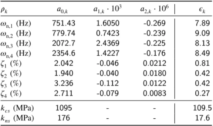
characteristics are given in Table2. The uncertainty bound was determined by calculating the standard deviation (𝜎) of the fitted parameters around the mean, which gave the±3𝜎 gray region in Fig.5. The uncertainty region was assumed to be independent of the spindle speedΩ. This results in Δ𝑘 ∈ ℝ,𝑘 = 1, ...,8, scalar parametric uncertainties, that can be included in the pseudospectral method. SinceΔ𝑘is a normalized variable (|Δ𝑘|<1), the weight𝜖𝑘is introduced to represent the actual scaling of the uncertain parameters.
Let𝜌𝑘be one of the parameter under considerations (given in Table2for this specific case), then its perturbed value can be written as𝜌𝑘+ Δ𝑘𝜖𝑘. The weights𝜖𝑘can be used to con- struct the scaling matrices𝐃𝑖𝑘and𝐄𝑖𝑘in (31). The list of the speed-dependent modal parameters and their uncertainties determined from experiments are given in Table2. The cut- ting force characteristics were identified from preliminary cutting tests, where the tangential and radial cutting coeffi- cients𝑘𝑐𝑠 and𝑘𝑛𝑠were both assumed to have 10%relative uncertainty. The uncertainties of the modal parameters were
4
3 4
^3
3 3
^2
3 2
^1
3 1
^n,4 Hz
n,4 Hz
3
^n,3 Hz
n,3 Hz
3
^n,2 Hz
n,2 Hz
3
^n,1 Hz
n,1 Hz
3
1 (%)2 (%)3 (%)4 (%)
n,4 (Hz)n,3 (Hz)n,2 (Hz)n,1 (Hz)
b a
, spindle speed (rpm) 5000 7000 9000 11000 13000 0
2 4 6
, spindle speed (rpm) 5000 7000 9000 11000 13000 0
2 4 6
, spindle speed (rpm) 5000 7000 9000 11000 13000 0
2 4
1 3 5
, spindle speed (rpm) 5000 7000 9000 11000 13000 0
2 1 3 4
, spindle speed (rpm) 5000 7000 9000 11000 13000
, spindle speed (rpm) 5000 7000 9000 11000 13000
, spindle speed (rpm) 5000 7000 9000 11000 13000
, spindle speed (rpm) 5000 7000 9000 11000 13000 2320
2340 2360 2380
2040 2060 2080 2100
720 740 760 800 780
700 720 740 780 760
^
Figure 5: Change of modal parameters along the spindle speed.
(a) Natural frequencies (b) Damping ratios. Black dots de- note the fitted modal parameters, dashed curves are the fitted characteristics and gray region is the constant±3𝜎uncertainty region around the fitted mean.
Table 2
Change of the parameters along the spindle speed (𝜌𝑘(Ω) = 𝑎0,𝑘+𝑎1,𝑘Ω +𝑎2,𝑘Ω2,Ω ∈ [5000,13000]rpm) and their (addi- tive) uncertainty (𝜖𝑘 is independent fromΩ).
𝜌𝑘 𝑎0,𝑘 𝑎1,𝑘⋅103 𝑎2,𝑘⋅106 𝜖𝑘
𝜔n,1 (Hz) 751.43 1.6050 -0.269 7.89
𝜔n,2 (Hz) 779.74 0.7423 -0.239 9.09
𝜔n,3 (Hz) 2072.7 2.4369 -0.225 8.13
𝜔n,4 (Hz) 2354.6 1.4227 -0.176 8.49
𝜁1 (%) 2.042 -0.046 0.0212 0.81
𝜁2 (%) 1.940 -0.040 0.0180 0.42
𝜁3 (%) 3.236 -0.112 0.0122 0.42
𝜁4 (%) 2.711 -0.079 0.0083 0.27
𝑘𝑐𝑠(MPa) 1095 - - 109.5
𝑘𝑛𝑠 (MPa) 176 - - 17.6
chosen to be equal to the 3𝜎deviation, see Fig.5and the last row of Table2. Note, that variation in the modeshapes𝐔𝑙 are difficult to measure and are often neglected (see [30]). In this study we also assume that the modeshapes do not change and no uncertainty is added.
The stability lobe diagrams corresponding to machining parameters given in Table3can be seen in Fig.6(b), where dashed curves denote the stability boundaries obtained by neglecting speed dependency (modal parameters in Table1), and solid black curves are the boundaries obtained by the speed-dependent parameters in Table2. Fig.6(a) presents the strengths of the harmonics of the chatter vibrations that can be calculated from the dominant eigenvalue and the Fourier
Table 3
Machining parameters.
Tool Workpiece
Al2024-T351 Process
𝑍𝑡=2 𝑘𝑐𝑝=16 N/mm 50% down-milling 𝐷=16 mm 𝑘𝑐𝑠=1095 MPa 𝜑en=90◦ 𝛾 =30◦ 𝑘𝑛𝑝=34 N/mm 𝜑ex=180◦
𝑘𝑛𝑠=176 MPa 𝑓𝑧 =0.1 mm/tooth
transform of the corresponding eigenvector, see the method presented in [18]. In panel (a) black denotes the dominant chatter frequency𝜔c,d, while gray shading indicates the other harmonics with less energy. This diagram is used to identify the dominant frequencies from measurements.
The robust stability lobe diagram was determined us- ing the pseudospectral method. During the calculations, ten parametric uncertainties were assumed with weights given in the last column of Table2.
Experimental chatter tests were carried out with fine res- olution from spindle speed 5000 rpm to 13000 rpm. Ac- celerometers were mounted onto the workpiece and spindle housing, moreover a microphone was also placed close to the machining area. Chatter was identified based on the spectra of the signals measured during cutting. Each measured point in panel (a) was marked by a filled circle if the operation was stable, by a cross if it was unstable, and by a triangle if chatter was not clearly identifiable. When the operation was unsta- ble, the dominant chatter frequency was selected and it was marked in Fig.6(a), also by a cross. For quantitative chatter indicators obtained from the cutting force and acceleration signals, we refer the reader to the method presented in [31].
Four sample spectra are given in Fig.6(c-f), which were captured by an accelerometer mounted on the spindle hous- ing in direction𝑦. Panels (c-d) are measured at spindle speed 7600 rpm, with depth of cut 0.75 and 1 mm. From the signal of the accelerometer the spectrum of the velocity𝑣𝑦was cal- culated and the dominant peaks were compared to the pre- dicted chatter frequencies. The absolute value of the FFT of the signal is indicated by dark gray curves, while dashed and point-dotted vertical lines indicate the tooth-passing fre- quencyftp = 60∕(𝑍𝑡Ω), its half, and their integer multi- plies. The dominant chatter peak and the shifted harmonics are colored by black. It can clearly be seen in panel (d) that the dominant chatter frequency occurs at 2204 Hz, which is close to the third vibration mode. A similar test is shown in panels (e-f), where tests were carried out at speed 12000 rpm, at depth of cuts were 1 and 1.5 mm. The dominant chat- ter frequency was identified at 724 Hz, close to the predicted first mode.
Although small uncertainties were assumed initially in the model, the robust stable maximum depth of cuts at the lowest points decrease by nearly 30%. On the other hand by measuring the vertical differences, a 0.15–1 mm wide uncer- tainty band can be observed, which is also significant.
Experiments show a qualitatively good agreement with the predictions, but not all of the points inside the robust
(b)
(d)
(f) (c)
(e)
ap = 1 mm = 7600 rpm ap = 0.75 mm
= 7600 rpm
ap = 1.5 mm = 12000 rpm ap = 1 mm
= 12000 rpm
unstable
C B D
A
D C B A
724 Hz 1125 Hz
1525 Hz
2325 Hz 1951 Hz
2204 Hz 2458 Hz
ftp
ftp
ftp
ftp n,3
n,4
1925 Hz Shifted
Original Robust
Unstable Stable Marginal
n,1 n,2
(a)
dominant chatter frequency
dominant chatter frequency stable
unstable
stable
unstable
yyyy
0.91 3.02
Figure 6: Calculated and measured stability lobe diagrams. (a) Dominant chatter frequencies obtained by calculations (continuous gray-shaded curves indicate the magnitude of frequency components along the stability boundaries) and observed in experiments (black crosses); (b) Stability diagrams: dotted – speed-independent modal parameters, solid – speed-dependent modal parameters, gray-shaded – robust stable; (c-f) FFTs of measured velocity signals corresponding to points A-B-C-D in panel (b).
stable domain were indeed stable during the chatter tests.
This indicates that there are still modeling errors and uncer- tainties present, which can explain this discrepancy. Possi- ble reasons can be the linear force characteristics used dur- ing calculations or the dynamical model with proportional damping which are simplifications of reality. On the other hand the run-out of the tool, nonlinearities and stochastic effects may also have a strong impact on the stability bound- aries.
6. Comparison with the MFS-SSV method
There exist several statistical methods in the literature to approximate the probability of stability if the probabil- ity density function of the uncertain parameters is known.
However, there are only a few methods that guarantee sta- bility if only upper and lower bounds on parameter values are available. These techniques are all called robust meth- ods, such as the approach inferred from the Edge Theorem [13], the structured singular value analysis [14] or the pseu- dospectral method. These approaches cannot determine the probability of stability, but the calculation is typically less time-consuming.
The Edge Theorem is applied to time-invariant models in [13], but the extension to time-periodic systems is not straightforward, because the characteristic equation cannot be determined in a similar way. It also requires an affine de-
pendence of the (scalar) characteristic equation on the uncer- tain parameters. The Multi-frequency Solution with Struc- tured Singular Value analysis (MFS-SSV, [14]) provides an alternative way to assess the robust stable region, but this method also has drawbacks. It is only applicable to modal parameter uncertainties, and the approximations of robust stable regions can be more conservative than others. In this section we assume that only the modal parameters are un- certain (Table2.) and compare the results obtained by the pseudospectral method and the MFS-SSV approach.
The Multi-frequency Solution of [32] can directly be ap- plied to the measured frequency response functions𝐇(𝜔) without parameter identification. This technique has been extended in [14] in order to consider additive uncertainties in the FRFs in the form𝐇(𝜔) +𝛿𝐇(𝜔), where𝛿𝐇(𝜔)is a complex-valued uncertainty. The structured singular value analysis assumes that the uncertainty can be restructured into a block-diagonal matrix𝚫̂, such that the governing equation is written as
det(
𝐈−𝐌(𝑎̂ p,Ω, 𝜔c)𝚫̂)
= 0, (40)
where𝐌,̂ 𝚫̂ ∈ℂ2(2𝑟+1)×2(2𝑟+1)are constructed according to [14], and𝑟is the highest number of harmonics considered during the expansion. The system is not robust stable if the determinant in (40) is zero for some𝚫̂ and𝜔c. The compu- tational algorithm presented in [14] gives a lower bound on
![Figure 3: Configuration and devices used during the experiment. The detailed specifications of the laser sensor and ball shooter gun are presented in [27].](https://thumb-eu.123doks.com/thumbv2/9dokorg/787498.36621/7.892.82.810.88.328/figure-configuration-devices-experiment-detailed-specifications-shooter-presented.webp)