CLUSTER ANALYSIS OF MULTICRITERIA-CLASSIFIED WHEELED ARMORED VEHICLES
KEREKES HARCJÁRMŰVEK TÖBBSZEMPONTÚ ÉRTÉKELÉSÉNEK KLASZTERANALÍZISE
GÁVAY, György; TÓTH, Bence
(ORCID: 0000-0003-0632-5650); (ORCID: 0000-0003-3958-187X) gavay.gyorgy@uni-nke.hu; toth.bence@uni-nke.hu
Abstract
Cluster analysis was performed on the data representing the defense of 32 wheeled armored vehicles based on a Multi Criteria Decision Support model. The number of clusters was determined by nonhierarchical clustering, while the vehicles were assigned to a cluster by non-hierarchical clustering. The number of clusters are either three or eight. For three assumed clusters, the BTR-type, the equipment designed before and after 2000 were grouped together, while for eight assumed clusters, these groups split into subgroups. Each subgroup consist of vehicles with similar defense, while the distinction between the subgroups could be made on the basis of modernization, the evolution of defense techniques in time.
Keywords: clustering, cluster analysis, k-means, GAIA, wheeled armored vehicle
Absztrakt
Harminckét kerekes harcjárművet jellemző, többszempontú döntéshozatali modell alapján kapott, a járművek védettségét leíró adatokon végeztünk klaszteranalízist. Hierarchikus módszerrel meghatároztuk a klaszterek számát, majd nemhierarchikus módszerrel az egyes klaszterek tagjait. A klaszterek lehetséges számára három és nyolc adódott.
Három feltételezett klaszter esetén a BTR típusú, a 2000 előtt, illetve után tervezett harcjárművek alkottak egy-egy csoportot, míg nyolc feltételezett klaszter esetén ezen három csoport részhalmazai alkottak egy-egy alcsoportot. Az alcsoportok közel azonos védettségű harcjárműveket tartalmaztak, míg az egyes csoportok között a védelem módjainak időbeli fejlődése, a modernizáció volt a legalapvetőbb különbség.
Kulcsszavak: klaszteranalízis, k-közép, GAIA, kerekes harcjármű
A kézirat benyújtásának dátuma (Date of the submission): 2019.02.14.
A kézirat elfogadásának dátuma (Date of the acceptance): 2019.04.11.
INTRODUCTION
The comparison, evaluation and ranking of armaments, and especially military equipment is an ever important task for every army [1][2]. Theoretical and practical analyses play an important role in the acquisition of wheeled armored vehicles which means the evaluation and the choosing from possible alternatives on the basis of several different criteria [3][4]. Proper Multi Criteria Decision Making (MCDM) models [5] give support for the theoretical analysis: with their help, the alternative choices can be ranked and their similarities and dissimilarities can be detected on the basis of a given set of criteria [6].
Furthermore, the results obtained by one method can be analyzed by another method, too.
This paper presents the cluster analysis of previous results [7] obtained by an MCDM model using the Visual PROMETHEE software [8]. This method has already been proved to be a sufficient tool for analyzing military equipment [9] The authors hope, that it can be utilized in the future in the field of comparative analysis of military equipment and military vehicles [10][11].
METHODS The PROMETHEE and GAIA methods
The data analyzed in this study was obtained by the PROMETHEE and the GAIA methods, which are described in detail in [12]. The GAIA method can visualize the alternatives and the criteria for the evaluation of the data processed the PROMETHEE model [12;pp.49-69].
The PROMETHEE method is capable to compare and rank a high number of alternatives.
The aim of our recent research, the results of which are used as the initial data of this study, was to compare and rank a total of 32 Armored Personnel Carriers (APC) and Infantry Fighting Vehicles (IFV).
At first, each criterion has to be weighted regarding its importance in the decision to be made.
This is the most vital, and also the hardest task to do, and it is based on the knowledge and experience of the decision maker. If done properly, not only the optimal choice from the alternatives but also the order between the alternatives can be obtained. The sum of the weights has to be 1.
Then, each alternative is described by a real number in the light of every criterion. By taking the weights into account, this results in having a 30-dimensional vector describing each alternative. To compare the alternatives, these vectors are projected from the 30-dimensional Euclidean space into a two-dimensional plane called GAIA-plane. This is carried out to lose as little information as possible, though some is inevitable. The difference between the original and the projected vectors can also be described by a vector, δj, for each alternative (1 ≤ j ≤ 32).
The PROMETHEE method makes projection to minimize the sum of the δjδj dot products
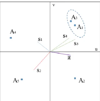
Figure 1. Example showing the projection of criterion vectors, alternatives and the Decision Stick on the GAIA plane. (Made by authors using [12].)
From the GAIA plane, the following information can be deduced:
̶ criteria with approximately parallel vectors can be satisfied simultaneously by the given alternatives,
̶ if two criteria are independent, they are represented by perpendicular vectors,
̶ two criteria, with vectors pointing in opposite directions cannot be satisfied simultaneously,
̶ the length of a criterion vector represents the distinctive power of the given criterion,
̶ alternatives closer to a vector mean a better choice in fulfilling that criterion, while alternatives farther mean a worse choice.
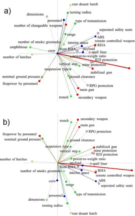
Two planes were used according to two applications area: the suitability for areal defense (AD) and the applicability in (abroad) mission field (MF). As a result, two full PROMETHEE rankings (Table1) and two GAIA planes were obtained. The criteria used for each application can be seen in Figure2. The red vector is the Decision Stick.
Figure 2. Visualization of the criteria on the GAIA plane for the a) AD and the b) MF applications. The Decision Stick is indicated by the thick red line. (Made by authors.)
AD alternative Phi Phi+ Phi- MF alternative Phi Phi+ Phi- 1 Patria AMV xp 0.2692 0.3085 0.0393 1 Patria AMV_XC360P 0.2279 0.2733 0.0454 2 Patria AMV 0.2677 0.3032 0.0355 2 Pandur_II 8x8 0.2145 0.2658 0.0513 3 Patria AMV_XC360P 0.2572 0.2977 0.0405 3 Pandur_II 6x6 0.2119 0.2755 0.0636 4 Piranha 5 0.2455 0.2908 0.0453 4 Patria AMV 0.2097 0.2687 0.059 5 Pandur_II 8x8 0.2287 0.2799 0.0511 5 Patria AMV xp 0.2089 0.269 0.0601 6 VBCI_I 0.2144 0.2641 0.0497 6 Piranha 5 0.2 0.2574 0.0574 7 VBCI_II 0.2092 0.2685 0.0593 7 VBCI_I 0.1831 0.235 0.0519 8 FSNN 8x8 0.1924 0.2285 0.0361 8 FSNN 8x8 0.179 0.2302 0.0511 9 Boxer IFV 0.1533 0.2761 0.1228 9 VBCI_II 0.1583 0.2359 0.0776 10 Pandur_II 6x6 0.1461 0.2214 0.0753 10 VAB_II 0.1524 0.2224 0.07 11 VAB_III 0.1388 0.2251 0.0863 11 Boxer APC 0.1392 0.2414 0.1022 12 VAB_II 0.1339 0.2087 0.0748 12 Ejder 0.1387 0.2086 0.07 13 Ejder 0.1261 0.188 0.0619 13 Boxer IFV 0.1211 0.2631 0.142 14 FSNN 6x6 0.0943 0.1653 0.071 14 VAB_III 0.1129 0.1968 0.0839 15 BTR 90 0.0717 0.2556 0.1839 15 FSNN 6x6 0.0716 0.1624 0.0908 16 Boxer APC 0.065 0.2136 0.1486 16 Stryker DVH 0.0487 0.1718 0.1231 17 Stryker DVH 0.0047 0.1656 0.1608 17 BTR 90 0.0145 0.2363 0.2218 18 LAV25 0.0008 0.1822 0.1814 18 Fuchs_II -0.014 0.154 0.168 19 M1117 TAPV -0.0314 0.15 0.1814 19 LAV25 -0.0418 0.1733 0.2151 20 Fuchs_II -0.0481 0.1618 0.2099 20 M1117 TAPV -0.064 0.1439 0.2079 21 BTR 82A -0.0494 0.1963 0.2457 21 VAB NG -0.1235 0.1467 0.2702 22 Patria XA185 -0.08 0.1419 0.2218 22 BTR 82A -0.1267 0.1697 0.2964 23 VAB NG -0.1986 0.1144 0.313 23 Piranha III -0.1291 0.1108 0.2399 24 Fuchs_A8 -0.204 0.1137 0.3178 24 Patria XA185 -0.1504 0.1267 0.2772 25 Piranha III -0.2061 0.0905 0.2967 25 Fuchs_A8 -0.1695 0.128 0.2975 26 BTR 80A -0.235 0.1402 0.3752 26 Pandur_I -0.1782 0.1277 0.3059 27 Pandur_I -0.2513 0.0906 0.3418 27 VAB_I -0.1794 0.1328 0.3122 28 Patria XA202 -0.2673 0.0675 0.3348 28 M1117 ASV -0.26 0.0492 0.3092 29 VAB_I -0.2788 0.0936 0.3724 29 Patria XA202 -0.2806 0.0838 0.3643 30 M1117 ASV -0.3153 0.0387 0.3539 30 Fuchs_I -0.2888 0.0696 0.3584 31 Fuchs_I -0.3249 0.0585 0.3834 31 BTR 80 -0.2911 0.1006 0.3917 32 BTR 80 -0.329 0.0825 0.4115 32 BTR 80A -0.2953 0.1212 0.4165 Table 1. The PROMETHEE ranking of equipment in the AD and MF applications. (Made by authors from
the results of Visual PROMETHEE Academic Free Edition1 [13][14].)
Clustering methods
To determine the clusters of data points, two types of clustering have to be carried out: first, a hierarchical clustering to obtain the number of clusters and then a non-hierarchical one to get the exact elements of the clusters. All of the clustering was carried out in the R programming language and environment [15].
1 The Visual PROMETHEE Academic Edition is fully functional without any limits. It is available for free for non-profit research and teaching only.
Hierarchical clustering
For the hierarchical clustering, agglomerative methods were used. These methods start with as many clusters as data points: each data point is one cluster. The distance between each pair of clusters is determined and the two clusters with minimal distance are merged into a new cluster.
Then the distances between the new clusters are determined again, and the two with minimal distance are merged again and this process goes on until every data point belongs to one cluster.
This means that in each step the number of clusters decreases by one and there are (N – 1) steps in the clustering process.
The hierarchical clustering was carried out by using the hclust() function of the built-in stats package [15] of R. The methods selected to determine the distance between clusters were:
̶ the Single Linkage Method,
̶ the Complete Linkage Method,
̶ the Average Linkage Method (also known as UPGMA, Unweighted Pair Group Method with Arithmetic averaging) and
̶ the McQuitty Method (or WPGMA, Weighted Pair Group Method with Arithmetic averaging).
The selection was made to ensure that at each step the distance measure increases and thus a sudden increase in the minimal distance of the two clusters merged in the mth step is a sign of having reached the optimal number of clusters in the (m ‒ 1)th step. In other words, denoting the distance between the two closest clusters in the mth step by ℓm, if ℓm ‒ ℓm-1 ≫ ℓm-1 ‒ ℓm-2, then the optimal number of clusters is (m ‒ 1).
There are several possible metrics to use to determine the distance. In this study, the most common one, the Euclidean distance was used.
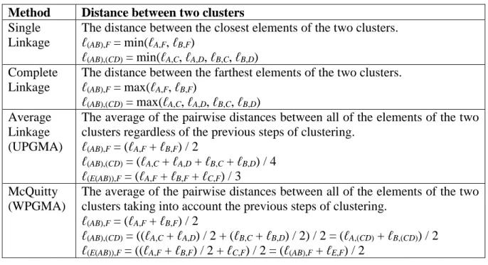
The clustering methods differ in how they calculate the distance of two clusters at least one of which contain more than one element. To demonstrate these differences, let a = (AB) denote the cluster of data points A and B, (C(AB)) or ((AB)C) denote the merged cluster of (AB) and data point C. The distance between data points A and B, between clusters (AB) and (CD) and between cluster (AB) and data point C will be denoted by ℓA,B, ℓ(AB),(CD) and ℓ(AB),C, respectively. The mean value of the coordinates of the data points in cluster a, called centroid, is denoted by ā and for a merged ab cluster by 𝑎𝑏̅̅̅. The distances calculated by each method is summarized in Table 1. [8]
Method Distance between two clusters Single
Linkage
The distance between the closest elements of the two clusters.
ℓ(AB),F = min(ℓA,F, ℓB,F)
ℓ(AB),(CD) = min(ℓA,C, ℓA,D, ℓB,C, ℓB,D) Complete
Linkage
The distance between the farthest elements of the two clusters.
ℓ(AB),F = max(ℓA,F, ℓB,F)
ℓ(AB),(CD) = max(ℓA,C, ℓA,D, ℓB,C, ℓB,D) Average
Linkage (UPGMA)
The average of the pairwise distances between all of the elements of the two clusters regardless of the previous steps of clustering.
ℓ(AB),F = (ℓA,F + ℓB,F) / 2
ℓ(AB),(CD) = (ℓA,C + ℓA,D + ℓB,C + ℓB,D) / 4 ℓ(E(AB)),F = (ℓA,F + ℓB,F + ℓC,F) / 3
McQuitty (WPGMA)
The average of the pairwise distances between all of the elements of the two clusters taking into account the previous steps of clustering.
ℓ(AB),F = (ℓA,F + ℓB,F) / 2
ℓ(AB),(CD) = ((ℓA,C + ℓA,D) / 2 + (ℓB,C + ℓB,D) / 2) / 2 = (ℓA,(CD) + ℓB,(CD)) / 2 ℓ(E(AB)),F = ((ℓA,F + ℓB,F) / 2 + ℓC,F) / 2 = (ℓ(AB),F + ℓE,F) / 2
Table 2. The calculation of the distance of two clusters by each criterion (made by authors)
Non-hierarchical clustering
Knowing the number of expected clusters from the hierarchical method(s), non-hierarchical clustering can be carried out to determine the members of each cluster. For this purpose, the so-called k-means clustering will be used. A metric is also needed, with which the distances are determined, for which the Euclidean distance was used.
First, k so-called centroid points are randomly selected on the plane and each data point is assigned to the closest centroid. Then, an iteration process is carried out to determine the best positions for the centroids:
̶ the position of the centroid of each cluster is recalculated by taking the mean value of the coordinates of the data points assigned to that cluster,
̶ if the positions of the centroids did not change, end the iteration,
̶ if the positions of the centroids changed, assign the data points to the cluster of the closest, newly calculated centroid.
In case of the Euclidean distance, the k-means method always converges. However, the exact assignment of data points to clusters can depend on the initial choice of the centroids, therefore several consecutive runs of the clustering algorithm have to be carried out. In our case, 1000 consecutive runs with different starting centroids were done.
Let us denote the distance between data point xi and centroid cj, with d(xi, cj), where 1 ≤ j ≤ k. By the nature of the clustering method, the minimum of this function is for the centroid of the cluster of xi:
min𝑗 𝑑(𝑥𝑖; 𝑐𝑗) (1)
The so-called sum of squared errors (SSE) is calculated as the sum of the squares of the distances of the data points to their respective centroids:
𝑆𝑆𝐸 = ∑ (min
𝑗 𝑑(𝑥𝑖; 𝑐𝑗))
𝑁 2
𝑖=1 , (2)
where N is the total number of data points. The clustering with the lowest SSE value is chosen to be the valid clustering.
The k-means clustering was carried out by using the KMeans_rcpp() function of the ClusterR package [16]
RESULTS AND DISCUSSION
Without any clustering performed, it can be stated in general that the farther to the right an equipment is on the plane (i.e. closer to the Decision Stick), the more modern it is (see Fig. 4).
Hierarchical clustering
Performing the hierarchical clustering with the four methods on the data of both the AD and the MF GAIA planes, the same results were obtained. The change in the minimal distance that determines which clusters to merge, shows two steps: one between 2 and 3 clusters and one between 7 and 8 clusters for the Single Linkage, Average Linkage and McQuitty methods (see Fig. 3). There is no significant change in the behavior of the distance measure in case of the Complete Linkage method. This means that there are either 3 or 8 reasonable clusters in the data set. Therefore, the k-means clustering was carried out for these two k values.
0 500 1000 1500 2000 2500
Min im a l d is ta n c e ( a .u .)
At first sight, the GAIA plane regarding the MF application area differs from the GAIA plane regarding the AD application area in that the criterion vectors and alternatives are approximately mirrored to the horizontal axis. In fact, this does not have any practical relevance on the clustering because only the relative positions of alternatives and criteria vectors have to be taken into consideration. Since these relative positions are mostly the same in the two application areas, the criteria have similar effects on the alternatives. Regarding the results, not only the similarities but also the differences are important.
Three clusters
The results of the k-means clustering for k = 3 assumed clusters can be seen in Figure 4.
Cluster A is the group of the four BTR vehicles, which have the most important distinctive property that they lack the rear hatch.
The distinction between clusters B and C can be made on the temporal base: the vehicles grouped together in cluster B were constructed much earlier than the ones in cluster C. All of the ones belonging to cluster B were designed before 2000, while the ones belonging to cluster C were developed after 2005. The two clusters thus distinguish the vehicles from the 20th and the 21st century.
The Decision Stick aims at the right side of cluster C, which area contains the group of the alternatives that best satisfy the defense criteria.
These observations are also valid for the respective D, E and F clusters.
a)
C A
B
M1117 TAPV FNSS 8x8
Stryker DVH
Pandur II 8x8
VBCI I Patria AMV
Patria AMV XC 360 BOXER IFV
Patria AMV XpPiranha 5 VBCI II BOXER APC Pandur II 6x6
FNSS6x6 Ejder
VAB III VAB II Fuchs II
LAV 25
M1117 ASV Patria XA 202 Piranha III Fuchs A8 VAB NG
Fuchs I VAB I
Pandur I Patria XA 185
BTR 80
BTR 80A BTR 90
BTR 82A
b)
F
E D
M1117 TAPV
FNSS 8x8 Stryker DVH
Pandur II 8x8 VBCI I
Patria AMV Patria AMV XC 360
BOXER IFV Patria AMV Xp
Piranha 5 VBCI II
BOXER APC Pandur II 6x6
FNSS6x6 Ejder
VAB III VAB II LAV 25
M1117 ASV Patria XA 202
Piranha III VAB I
Pandur I Patria XA 185
BTR 80 BTR 80A
BTR 90 BTR 82A
Eight clusters
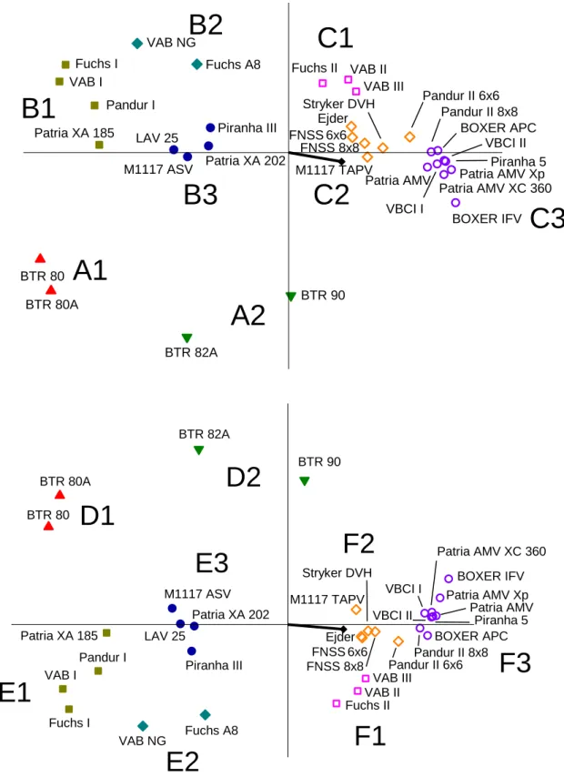
The results of the k-means clustering for k = 8 assumed clusters can be seen in Figure 5.
Figure 5. The k-means clustering of the data points of the alternatives on the a) AD and the b) MF planes. The clustering was performed 1000 times with k = 8. The black vector is the Decision Stick. (Made by
authors.)
A2 A1
C2 C3 C1
B3 B2 B1
M1117 TAPV FNSS 8x8
Stryker DVH
Pandur II 8x8
VBCI I Patria AMV
Patria AMV XC 360 BOXER IFV
Patria AMV XpPiranha 5 VBCI II BOXER APC Pandur II 6x6
FNSS6x6 Ejder
VAB III VAB II Fuchs II
LAV 25
M1117 ASV Patria XA 202 Piranha III Fuchs A8 VAB NG
Fuchs I VAB I
Pandur I Patria XA 185
BTR 80
BTR 80A BTR 90
BTR 82A
F3 F2
F1 E3
E2 E1
D2 D1
M1117 TAPV
FNSS 8x8 Stryker DVH
Pandur II 8x8 VBCI I
Patria AMV Patria AMV XC 360
BOXER IFV Patria AMV Xp
Piranha 5 VBCI II
BOXER APC Pandur II 6x6 FNSS6x6
Ejder
VAB III VAB II Fuchs II LAV 25
M1117 ASV Patria XA 202
Piranha III
Fuchs A8 VAB NG
Fuchs I VAB I
Pandur I Patria XA 185
BTR 80 BTR 80A
BTR 90 BTR 82A
In this clustering case, cluster A of Fig.4 splits into two parts. As previously mentioned, clusters B and C split on when the cluster members were designed. This is true for clusters A1 and A2: the BTR–82A and BTR–90 are slightly more recent developments, and thus somewhat better constructions than the BTR–80 and BTR–80A, though still far below the present standards.
Assuming eight clusters, cluster B of Fig.4 splits into three. Again, the newer, the better:
while the vehicles in the B1 cluster are the equipment of the 1970s and 1980s, the vehicles of cluster B2 are the modernized versions of those and cluster C1 contains the newest versions of these vehicles. Elements of cluster B3 are better than both B1 and B2, thus their distinction by the clustering algorithm is reasonable: their protection is better in all aspects.
Undoubtedly, cluster C3 is the cluster of the best protected vehicles in the data set. This is obvious from its position: it lies closest to the direction of the Decision Stick of the GAIA plane.
The elements of C1 are slightly inferior to them, mainly because of their construction: since they have less axles, the nominal ground pressure they expose is higher. The separation of cluster C2 can have two reasons: either the vehicle has lower ballistic defense capability, or they are much heavier than the vehicles with similar other aspects in cluster C2, which is an important criterion in the ranking process. The only exception is the M1117 TAPV, which is well defended and small. It is nicknamed “pitbull”, but in this ranking its larger weight and size seems to be a slight disadvantage due to the smaller number of soldiers it can carry. A similar exception in the cluster C2 the Pandur II 6x6 vehicle which could belong to cluster C3, but it has small payload capability.
CONCLUSION
Based on the data of a Multi Criteria Decision Making model and hierarchical and non-hierarchical clustering, we have shown that the different types of wheeled armored vehicles with similar level of protection tend to group together on the GAIA plane both in the areal defense and abroad mission field application areas.
If the evaluation of a new equipment, based on the same criteria, is carried out and its resulting data point is projected on the two GAIA planes presented, it can be compared to the ones already analyzed. This can provide suggestions regarding which equipment the new one is similar to (as a substitute alternative) or better or worse than the others according to the criteria taken into account.
REFERENCES
[1] GYARMATI, J.: Napjainkban alkalmazott irányított páncéltörő rakétarendszerek összehasonlító elemzése; Katonai Logisztika 20. 3. (2012), pp. 57-72. (in Hungarian), URL:
[4] GYARMATI, J.: Haditechnikai eszközök összehasonlítása közbeszerzési eljárás során;
Hadmérnök I. 2. (2006), pp. 68-93., URL:
http://hadmernok.hu/archivum/2006/2/2006_2_gyarmati.pdf, last accessed: 11.02.2019.
[5] GYARMATI, J.: Military Application of Multi-Criteria Decision Making; Academic and Applied Research in Military and Public Management Science 14. 4. (2015), pp. 291- 297., URL: https://folyoiratok.uni-nke.hu/document/uni-nke-hu/aarms-2015-4- gyarmati.original.pdf, last accessed: 11.02.2019.
[6] GYARMATI, J.: Haditechnikai eszközök összehasonlítása: útmutató; Zrínyi Miklós Nemzetvédelmi Egyetem, Budapest, Hungary, 2011. (in Hungarian)
[7] GÁVAY, Gy.: Kerekes harcjárművek védettségének vizsgálata és összehasonlító elemzése az elmúlt évtizedek katonai tapasztalatainak és követelményeinek felhasználásával, PhD thesis, in progress (in Hungarian)
[8] http://paleodb.org/public/summercourse07/olszewski_clustering.pdf, last accessed:
11.02.2019.
[9] GYARMATI, J.; FELHÁZI, S.; KENDE, Gy.: Choosing the Optimal Mortar for an Infantry Battalion's Mortar Battery with Analytic Hierarchy Process using Multivariate Statistics; In: NATO (szerk.) Decision Support Methodologies for Acquisition of Military Equipment, Brussels, Belgium: NATO Research and Technology Organisation (RTO), (2009), pp. 1-12
[10] GYARMATI, J.; VÉG, R. L.; HEGEDŰS, E.; GÁVAY, Gy. V.: A katonai felsőoktatás részvételének lehetőségei a kutatás-fejlesztési folyamatokban; Műszaki Katonai Közlöny XXVIII. 1. (2018), pp. 193-208 (in Hungarian) URL: http://hhk.archiv.uni- nke.hu/downloads/kiadvanyok/mkk.uni-nke.hu/PDF_2018_1sz/13_Gyarmati-Vegh- Hegedus-Gavay_Oktatas%20MKK%20cikk.pdf, last accessed: 11.02.2019.
[11] GÁVAY, Gy.; GYARMATI, J.; HEGEDŰS, E.; VÉG, R. L.: A kutatás fejlesztés szerepe és hatása az oktatásra az NKE HHK Haditechnikai tanszékén, Hadmérnök XII:(4) (2017), pp. 26-33 (in Hungarian), URL: http://hadmernok.hu/174_03_gavay.pdf, last accessed:
11.02.2019.
[12] RAPCSÁK, T.: Többszempontú döntési problémák; Budapesti Corvinus Egyetem, Budapest, Hungary, 2007.
[13] http://www.promethee-gaia.net/software.html, last accessed: 11.02.2019.
[14] http://www.promethee-gaia.net/files/VPManual.pdf, last accessed: 11.02.2019.
[15] R Core Team (2012). R: A language and environment for statistical computing. R Foundation for Statistical Computing, Vienna, Austria. ISBN 3-900051-07-0, URL http://www.R-project.org/
[16] MOUSELIMIS, L.: ClusterR: gaussian mixture models, K-Means, mini-batch-Kmeans and K-Medoids clustering. https://CRAN.R-project.org/package=ClusterR, R package version 1.1.8