Optimal partisan districting on planar geographies

(1)

Optimal partisan districting on planar geographies

Attila Tasn´adi

MTA-BCE “Lendület” Strategic Interactions Research Group, Department of Mathe- matics, Corvinus University of Budapest, H – 1093 Budapest, F˝ovám tér 8, Hungary, attila.tasnadi@uni-corvinus.hu

June 2013

Abstract. We show that optimal partisan districting in the plane with geographical constraints is an NP-complete problem.

Keywords: districting, gerrymandering, NP-complete problems.

(2)

1 Introduction

In electoral systems with single-member districts (or even with at least two multi- member districts) redistricting has to be carried out to resolve geographic malappor- tionment caused by migration and different district population growth rates. An in- herent difficulty associated with redistricting is that it may favor a party. The problem becomes even worse if redistricting is manipulated for an electoral advantage, which is referred to asgerrymandering.

In the middle of the previous century it was hoped that the problem of gerrymandering could be overcome by computer programs using only data on voters geographic distribution without any statistical information on voters preferences (e.g. Vickrey, 1961) and thus determining an ‘unbiased’ districting. The first algorithm finding all districtings with (i) equally sized, (ii) connected and (iii) compact districts was given by Garfinkel and Nemhauser (1970).¹ The computational difficulty of the problem was clear from the very beginning. Nagel (1972) documented in an early survey the computational limitations of automated redistricting by considering the available programs of his time. Altman (1997) showed that the problems of achieving any of the three mentioned criteria are NP-hard. Moreover, he also demonstrated that maximizing the number of competitive districts is also NP-hard. Because of the computational difficulty of the problem there is a growing literature on new approaches to finding unbiased districtings (see, for instance, Mehrotra et al. (1998), Bozkaya et al. (2003), Ba¸c˜ao et al. (2005), Chou and Li (2006), Ricca and Simeone (2008) or Ricca et al. (2008)). For recent surveys we refer to Ricca et al. (2011) and Tasndi (2011).

Though finding an equally sized districting is already computationally hard, from another point of view it is feared by the public that the continuously increasing computational power makes the problem of carrying out an optimal partisan gerrymandering possible. However, the underlying difficulty that hinders us in finding an unbiased districting, does not allow us to determine an optimal partisan redistricting. Indeed, Altman and McDonald (2010) provide recent evidence that current computer programs are far away from finding an optimal gerrymandering.

A formal proof establishing that a simplified version of the optimal gerrymandering problem is NP-complete was given by Puppe and Tasn´adi (2009). Though they take geographical constraints into account, planarity is not prescribed explicitly. The current paper overcomes this shortcoming by locating voters in the plane.

2 The Framework

We assume that parties A and B compete in an electoral system consisting only of single member districts. In addition, voters with known party preferences are located in the plane and have to be divided into a given number of almost equally sized districts.

The districting problem is defined by the following structure:

Definition 1. Adistricting problem is given by Π = (X, N,(x_i)_i∈N, v, K,D), where

• X is a bounded and strictly connected² subset ofR²,

1Earlier Hess et al. (1965) provided an algorithm striving for similar goals; however, their algorithm did not always obtain optimal solutions.

2We call a bounded subsetAofR²strictly connectedif its boundary∂Ais a closed Jordan curve.

(3)

• the finite set of voters is denoted byN ={1, . . . , n},

• the distinct locations of voters are given by x1, . . . , xn∈int(X),

• the voters’ party preferences are givenv:N → {A, B},

• the set of district labels is denoted byK={1, . . . , k}, wherebn/kc ≥3, and

• D denotes the finite set of admissible districts consisting of bounded and strictly connected subsets of X and each of them containing the location of bn/kc or dn/kevoters,³and furthermore,

• we shall assume that based on their locations thenvoters can be partitioned into k districts{D1, . . . , Dk} ⊆ D.

Observe that in defining the districting problem, we assumed that obtaining an almost equally sized districting is possible, which can be justified by the fact that finding an admissible districting for real-life problems is possible, while finding a districting satisfying additional requirements such as partisan optimality is difficult. In particu- lar, the staff hired to produce a districting map could always construct a districting map consisting of almost equally sized districts although other properties as partisan optimality are difficult to prove or confute. Producing a districting with almost equally sized districts, is a tractable problem if there are not to many geographical restrictions since we can obtain a result by drawing districts from left to right and from top to bottom on a map of a state by keeping the average district size in mind.

We shall mention that in reality the basic units of a districting problem from which districts have to be created are census blocks or counties rather than voters. In this case voter preferences v : N → {A, B} have to be replaced by a function of type v⁰ :N⁰ →[0,1], where N⁰ stands for the finite set of counties, expressing the fraction of partyAvoters. However, our results obtained in this paper can be extended to this more general setting, by allowing the case of almost equally sized counties, for which district outcomes are determined by the number of winning counties for partyA, which happens to be the case, for instance, ifv⁰(N⁰) ={α,1−α} for a givenα∈[0,1/2).

Turning back to our districting problem defined on the level of voters, we have to assign each voter to a district.

Definition 2. An f : N → D is a districting for problem Π if there exists a set of districtsD1, . . . , Dk ∈ Dsuch that

• f(N) ={D1, . . . , D_k},

• D_i∩D_j=∅ifi6=j andi, j∈K,

• {x_i|i∈f⁻¹(D_j)} ⊂int(D_j) for anyj∈K.

Observe that without loss of generality we do not explicitly require that a districting covers the entire country but just the inhibited areas.

Definition 3. Two districtingsf :N → D and g:N → D with districts D1, . . . , Dk

and D⁰₁, . . . , D⁰_k, respectively, are equivalent if there exists a bijection between the series of sets{xi|i∈f⁻¹(D1)}, . . . ,{xi |i∈f⁻¹(Dk)} and the series of sets{xi |i∈ g⁻¹(D⁰₁)}, . . . ,{xi|i∈g⁻¹(D⁰_k)}such that the respective sets are identical.

3bxcstands for the largest integer not greater thanx∈Randdxestands for the smallest integer not less thanx∈R.

(4)

Clearly, by defining equivalent districtings we have defined an equivalence relation above the set of districtings for problem Π.

A districtingf and voters’ preferencesv determine the number of districts won by partiesAandB, which we denote byF(f, v, A) andF(f, v, B), respectively. If the two parties should receive the same number of votes in a district, its winner is determined by a predefined tie-breaking ruleτ:D → {A, B}.

Definition 4. For a given problem Π and tie-breaking ruleτ a districtingf :N → D isoptimal for partyI∈ {A, B}ifF(f, v, I)≥F(g, v, I) for any districtingg:N→ D.

Note that due to the above defined equivalence relation the set of districtings has finitely many equivalence classes, there exists at least one optimal districting for each party.

3 Determining an optimal districting is NP-complete

We establish that even the decision problem associated with the optimization problem of determining an optimal partisan districting, i.e. deciding for a given districting problem Π whether there exists a districting with at least m winning districts for a party, say party A, is an NP-complete problem; we call this problem WINNING DISTRICTS. In order to prove this, we shall reduce the INDEPENDENT SET problem on planar cubic⁴graphs, a proven NP-complete problem (see Garey and Johnson; 1979, pp. 195), to WINNING DISTRICTS. The INDEPENDENT SET problem asks whether a given graphGhas a set of non-neighboring vertices of cardinality not less thanm.

Theorem 1. WINNING DISTRICTS is NP-complete.

Proof. Whether a districting possesses at leastmwinning districts for partyAcan be verified easily in polynomial time, and therefore WINNING DISTRICTS is in NP.

We establish that INDEPENDENT SET on planar cubic graphs reduces to WIN- NING DISTRICTS. We define the mapping that assigns to an arbitrary planar cubic graph a districting problem in two steps.

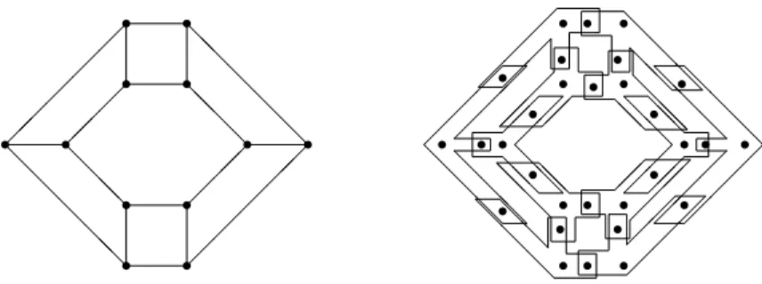
Step 1: We start with constructing partyA winning districts from a planar cubic graph G= (V, E). Let each vertex be a party A voter and replace the ‘midpoint’ of each edge with a party A voter. In addition, we associate with each vertex v ∈V a four member district containing the party Avoter assigned to vertex v and the three partyA voters replacing the three edges adjacent to vertexv. Hence, so far we have

|V|+|E|= 5|V|/2 partyA voters and|V| districts, where each of them is consisting of four partyAvoters. Step 1 is illustrated in Figure 1.

Observe that the given planar cubic graph has an independent set of size mif and only if we can select mdisjoint districts from the districts drawn in Step 1. However, as the right-hand side of Figure 1 shows, based on the districts drawn so far, we cannot partition the set of voters even if we extend the boundaries of the districts⁵in a way that the set of contained voters remains the same. Hence, we cannot obtain a districting.

This is what Step 2 takes care about.

Step 2: Now we associate with each district full of partyAvoters twelve new party B voters such that the new voters have to be placed on the ‘same side’ of the district as illustrated in Figure 2.

4A graph is cubic if the degree of each vertex equals 3.

5By extending districts appropriately we can assign any uninhabited area of a map to one district.

(5)

@

@@

@

@@r r r r r

r @

@

@@r r

r r

r

r r

r r r r

r r

r

r r r

r r

r

r r

r

@

@@

@

@@@

@

@@

@

@@@

@

@@

Figure 1: Associating party Awinning districts with a planar cubic graph

w w w

w

g g g g g g g g g g g g

Figure 2: PartyB voters

In addition, we have to form new districts distinguishing between the two cases whether a district full of partyA voters will be included in our districting. First, if a district full of partyAvoters is not selected by a districting, then the respective partyB voters should be grouped into partyB winning districts as shown in Figure 3. We will refer to these ‘vertical districts’ as type 1 partyBwinning districts. However, we have

w w w

w

Figure 3: Type 1 partyB winning districts

to be more careful since each of the three partyA voters corresponding to an edge of our initial planar cubic graphG= (V, E) is even a member of another partyAwinning district full of partyAvoters. Therefore, if none of these two districts containing the same party Avoter is contained in a districting, then this specific party A voter can be only included in one of these two type 1 districts. Hence, to make a districting possible we also include three type 2 ‘vertical districts’ associated with each partyA voter corresponding to an edge. Type 2 party B winning districts are illustrated in

(6)

Figure 4 in which the second partyAvoter from the left is a voter corresponding to a vertex of our initial planar cubic graph.

w w w

w

Second, if a district full of party A voters is selected by our districting, then the

‘horizontal districts’ illustrated in Figure 5 make a districting possible.

w w w

w

Observe that the districts introduced in Step 2 make a districting possible and that the given planar cubic graph has at least an independent set of sizem if and only if the associated districting problem has at leastm partyA winning districts.

It remains to be shown that given a planar cubic graph G= (V, E) its associated districting problem outlined in Steps 1 and 2 can be determined in polynomial time.

Constructing a straight line planar drawing of Gwith edges of at most five different slopes (see Keszeg et al. 2008) or a planar embedding in the grid of G(as shown by Liu et al. 1994), which can be obtained in polynomial time, we can easily locate the voters described in Steps 1 and 2 in the plane such that the respective districts can be drawn in polynomial time.

Remark 1. Considering our reduction, we can observe that the approximability of WINNING DISTRICTS cannot be better than that of INDEPENDENT SET on planar cubic graphs for which Burns (1989) showed that the approximation ratio of the polynomial time algorithm given by Choukhmane and Franco (1986) equals 7/8.

(7)

References

[1] M. Altman, Is automation the answer? The computational complexity of automated redistricting, Rutgers Computer and Law Technology Journal 23 (1997) 81–142.

[2] M. Altman, M. McDonald, The promise and perils of computers in redistricting, Duke Constitutional Law and Policy Journal 5 (2010) 69–112.

[3] F. Ba¸c˜ao, V. Lobo, M. Painho, Applying genetic algorithms to zone design, Soft Computing 9 (2005) 341–348.

[4] B. Bozkaya, E. Erkut, G. Laporte, A tabu search heuristic and adaptive memory procedure for political districting, European Journal of Operational Research 144 (2003) 12–26.

[5] J.E. Burns, The maximum independent set problem for cubic planar graphs, Net- works 19 (1989) 373-378.

[6] C-I. Chou, S.P. Li, Taming the gerrymander–statistical physics approach to political districting problem, Physica A 369 (2006) 799–808.

[7] E. Choukhmane, J. Franco, An approximation algorithm for the maximum independent set problem in cubic planar graphs, Networks 16 (1986) 349–356.

[8] M.R. Garey, D.S. Johnson, Computers and Intractability: A Guide to the Theory of NP-Completeness, W.H Freeman and Company, San Francisco, 1979.

[9] R.S. Garfinkel, G.L. Nemhauser, Optimal political districting by implicit enumer- ation techniques, Management Science 16 (1970) 495–508.

[10] S.W. Hess, J.B Weaver, H.J. Siegfeldt, J.N. Whelan, P.A. Zitlau, Nonpartisan political redistricting by computer, Operations Research 13 (1965) 998–1006.

[11] B. Keszegh, J. Pach, D. Pálvölgyi, G. Tóth, Drawing cubic graphs with at most five slopes, Computational Geometry 40 (2008) 138–147.

[12] Y. Liu, P. Marchioro, R. Petreschi, At most single-bend embeddings of cubic graphs, Applied Mathematics - A Journal of Chinese Universities 9 (1994) 127–

142.

[13] A. Mehrotra, E.L. Johnson, G.L. Nemhauser, An optimization based heuristic for political districting, Management Science 44 (1998) 1100–1114.

[14] S.S. Nagel, Computers & the law & politics of redistricting, Polity 5 (1972) 77–93.

[15] C. Puppe, A. Tasn´adi, Optimal redistricting under geographical constraints: Why

‘pack and crack’ does not work, Economics Letters 105 (2009) 93–96.

[16] F. Ricca, B. Simeone, Local search algorithms for political districting, European Journal of Operational Research 189 (2008) 1409–1426.

[17] F. Ricca, A. Scozzari, B. Simeone, Weighted Vornoi region algorithms for political districting, Mathematical Computer Modelling 48 (2008) 1468–1477.

(8)

[18] F. Ricca, A. Scozzari, B. Simeone, Political districting: from classical models to recent approaches, 4OR (2011) 223–254.

[19] A. Tasn´adi, The political districting problem: a survey, Society and Economy 33 (2011) 543–553.

[20] W. Vickrey, On the prevention of gerrymandering, Political Science Quarterly 76 (1961) 105–110.