Axiomatic Districting

(1)

Axiomatic districting

^*

Clemens Puppe¹ andAttila Tasn´adi²

1 Department of Economics, Karlsruhe Institute of Technology, D – 76131 Karlsruhe, Germany, clemens.puppe@kit.edu

2 Department of Mathematics, Corvinus University of Budapest, H – 1093 Budapest, F˝ov´am t´er 8, Hungary, attila.tasnadi@uni-corvinus.hu

June 2010

*The second author gratefully acknowledges financial support from the Corvinus University of Budapest through its Research Excellence Fellowship.

(2)

Summary. In a framework with two parties, deterministic voter preferences and a type of geographical constraints, we propose a set of simple axioms and show that they jointly characterize the districting rule that maximizes the number of districts one party can win, given the distribution of individual votes (the “optimal gerrymandering rule”). As a corollary, we obtain that no districting rule can satisfy our axioms and treat parties symmetrically.

Keywords: districting, gerrymandering.

JEL Classification Number: D72

(3)

1 Introduction

The districting problem has received considerable attention recently, both from the political science and the economics viewpoint. Much of the recent work has focused on strategic aspects and the incentives induced by different institutional designs on the political parties, legislators and voters (see, among others, Besley and Preston, 2007, Friedman and Holden, 2008, Gul and Pesendorfer, 2009). Other contributions have looked at the welfare implications of different redistricting policies (e.g. Coate and Knight, 2007). Finally, there is also a sizable literature on the computational aspects of the districting problem (see, e.g. Puppe and Tasn´adi, 2008, and the references therein).

In contrast to these contributions, the present paper takes a normative point of view. We formulate desirable properties (“axioms”) and investigate which districting functions satisfy them. There are several reasons for exploring this approach. First, the axiomatic method allows one to endow the vast space of conceivable districting rules with useful additional structure: each combination of desirable properties character- izes a specific class of districting rules, and thereby helps one to assess their respective merits. Second, one may hope that specific combinations of axioms single out a few, perhaps sometimes even a unique districting rule, thus reducing the space of possibili- ties. Finally, the axiomatic approach may reveal incompatibility of certain axioms by showing thatnodistricting rule can satisfy certain combinations of desirable properties, thereby terminating a futile search.

In a framework with two parties and geographical constraints on the shape of districts, we propose a set of simple axioms and show that they jointly characterize the districting rule that maximizes the number of districts one party can win, given the distribution of individual votes (the “optimal gerrymandering rule”). While some of the axioms have a more pragmatic justification, others have straightforward normative foundations such as the neutrality property which requires that a districting rule should treat parties symmetrically. Evidently, by generating a maximal number of winning districts for one of the parties, the optimal gerrymandering rule violates the neutrality axiom. Therefore, as a straightforward corollary of our main result, we obtain that no districting rule can satisfy a set of reasonable properties and treat parties symmetrically at the same time.

The work closest to ours in the literature is Chambers (2008, 2009) who also takes an axiomatic approach. However, one of his central conditions is the requirement that the election outcome beindependentof the way districts are formed (“gerrymandering- proofness”), and the main purpose of his analysis is to explore the consequences of this requirement. By contrast, our focus is precisely on the districting process which we try to structure by means of simple governing principles. In particular, geographical constraints which are absent in Chambers’ model play an important role in our analysis.

The districting rules that we consider depend among other things on the distribution of votes for each party in the population. One might argue, perhaps on grounds of some “absolute” notion ofex ante fairness, that a districting rule must not depend on voters’ party preferences since these can change over time. From this perspective, the districting problem is not really an issue and it would seem that any districting which partitions the population in (roughly) equally sized subgroups should be acceptable. By contrast, in the present paper we are interested in a “relative” orex post notion of fair districting, i.e. in the question of what would constitute an acceptable districting rule giventhe distribution of the supporters of each party in the population. This question

(4)

seems particularly important for practical purposes since a districting policy can be successfully implemented only if it receives sufficient support by theactual legislative body.

2 The Framework

We assume that parties A and B compete in an electoral system consisting only of single member districts, where the representatives of each districts are determined by plurality. The parties as well as the independent bodies face the following districting problem.

Definition 1 (Districting problem). A districting problem is given by the structure Π = (X,A, µ, µ_A, µ_B, t, G), where

• the voters are located within a subset X of the planeR²,

• A is the σ-algebra on X consisting of all districts that can be formed without geographical or any other type of constraints,

• the distribution of voters is given by a measureµon (X,A),

• the distributions of party A and partyB supporters are given by measures µA

andµB on (X,A) such thatµ=µA+µB,

• t is the given number of seats in parliament,

• G⊆ A, also called geography, is the set of admissible districts satisfying µ(g) = µ(X)/tand

µ_A(g)6=µ_B(g) (1)

for allg∈G, and possessing a partitioning ofX, i.e there exist mutually disjoint sets g⁰₁, . . . , g⁰_t∈Gsuch that∪^t_i=1g_i⁰=X.

Condition (1) excludes ties in the distribution of party supporters in all admissible districts to avoid the necessity of introducing tie-breaking rules. This condition is satisfied, for instance, if the set of voters is finite,µ, µA, µB are the counting measures and the district sizes are odd.

Definition 2 (Districting). A districting for the problem (X,A, µ, µA, µB, t, G) is a subsetD⊆Gsuch thatD forms a partition ofX and #D=t.

We shall denote byδA(D) and δB(D) the number of districts won by partyA and partyB under D, respectively. We write DΠ for the set of all admissible districtings of problem Π and letδ_A(D) ={δA(D) : D ∈ D}and δ_B(D) ={δB(D) :D ∈ D} for anyD ⊆ DΠ.

Definition 3 (Solution). A solution F associates to each districting problem Π a non-empty set of chosen districtingsF_Π⊆ D_Π.

(5)

3 Several Solutions

We now present a number of simple solution candidates. The first solution determines the optimal partisan gerrymandering from the viewpoint of partyA.

Definition 4 (Optimal solution for A). The optimal solutionO^A for party Adeter- mines for districting problem Π = (X,A, µ, µ_A, µ_B, t, G) the set of those districtings that maximize the number of winning districts for partyA, i.e.

O_Π^A= arg max

D∈DΠ

δA(D).

Evidently, in the absence of other objectives, O^A is the solution favored by party A supporters. The optimal solutionO^B for party B is defined analogously. If we are referring to an optimal solutionO, then we have eitherO^A orO^B in mind.

The next solution minimizes the difference in the number of districts won by the two parties. It has an obvious egalitarian spirit.

Definition 5(Most equal solution). The solutionMEdetermines for districting problem Π = (X,A, µ, µA, µB, t, G) the set of most equal districtings, i.e.

ME_Π= arg min

D∈DΠ

|δA(D)−δ_B(D)|. (2) Since an equal solution does not always exist the most equal solution aims to get as close as possible to equality in terms of the number of winning districts for the two parties.

The third solution maximizes the difference in the number of districts won by the two parties. The objective to maximize the winning margin of the ruling party could be motivated, for instance, by the desire to avoid too much political compromise.

Definition 6 (Most unequal solution). The solution MU determines for districting problem Π = (X,A, µ, µ_A, µ_B, t, G) the set of most unequal districtings, i.e.

MUΠ= arg max

D∈DΠ

|δA(D)−δB(D)|. (3) Fourth, we consider the solution that minimizes partisan bias. It has a clear motivation from the point of view of maximizing representation of the “people’s will” in the sense that the share of the districts won by each party is as close as possible to its share of votes in the population.

Definition 7(Least biased solution). The solutionLBdetermines for districting problem Π = (X,A, µ, µA, µB, t, G) the set of those districtings that minimize the absolute difference between shares in winning districts and shares in votes, i.e.

LB_Π= arg min

D∈DΠ

δ_A(D)

t −µ_A(X) µ(X)

= arg min

D∈DΠ

δ_B(D)

t −µ_B(X) µ(X)

. (4)

Finally, we mention the trivial solution that associates to each problem the set of alladmissible districtings.

Definition 8 (Complete solution). The complete solutionC associates with any districting problem Π = (X,A, µ, µA, µB, t, G) the set of all possible districtingsDΠ.

(6)

4 Axioms

In this section, we formulate five simple axioms each of which has an appeal either from a normative or a pragmatic point of view.

The case of two districts plays a fundamental role in our analysis. Note that by (1) it is not possible that a party can win both districts under one districting and lose both districts under another districting, i.e. if t = 2 then δA(DΠ) (respectively, δB(DΠ)) cannot contain both 0 and 2. Our first axiom requires that a solution must in fact be “determinate” in the two-district case in the sense that it must not leave open the issue whether there is a draw between the two parties or a victory for one party.

In other words, if a solution chooses a districting that results in a draw between the parties for a given problem it cannot choose another districting for thesameproblem that results in a victory for one party.

Axiom 1 (Two-district determinacy). A solutionF satisfiestwo-district determinacy if for any districting problem Π witht= 2, the setsδA(FΠ) andδB(FΠ) are singletons.

Evidently, all solutions considered in Section 2 with the exception of the complete solutionCsatisfy Axiom 1. Also observe that on the family of all two-district problems the most equal solutionME and the least biased solutionLB coincide.¹

Our next axiom requires that a solution behaves “uniformly” on the set of two- district problems in the sense that the solution must treat different two-district problems in the same way, provided they admit the same set of possible distributions of the number of districts won by each party.

Axiom 2 (Two-district uniformity). A solution F satisfiestwo-district uniformity if for any districting problems Π and Π⁰ with t= 2 such that δA(DΠ) =δA(DΠ⁰) (and therefore also δB(DΠ) = δB(DΠ⁰)) we have δA(FΠ) = δA(FΠ⁰) (and therefore also δB(FΠ) =δB(FΠ⁰)).

Even though it is imposed only in the two-district case, Axiom 2 is admittedly a strong requirement. It is motivated by the desire to keep the complexity of a solution manageable. Evidently, without Axiom 2, characteristics other than the possible distributions of the number of districts won by each party would have to enter the definition of a solution. Whatever these characteristics may be – whether derived from the underlying distribution of party supporters or from geographical information – their influence would complicate the definition and implementation of a districting rule con- siderably. In any case, it is easily seen that all solutions presented in Section 2 above satisfy Axiom 2.

Our third axiom, imposed on districting problems of any size, has a motivation similar to that of the previous axiom. It states that if a possible districting induces the same distribution of the number of winning districts for each party than some districting chosen by a solution, it must be chosen by this solution as well.

Axiom 3(Indifference). A solutionF satisfiesindifference if for any districting problem Π we have that D∈FΠ,D⁰ ∈ DΠ, δA(D) =δA(D⁰) andδB(D) =δB(D⁰) implies D⁰∈FΠ.

1To verify this, observe that if there exist admissible districtingsD, D⁰∈ DΠwithδA(D) = 2 and δA(D⁰) = 1, then one must have 0.5< µA(X)/µ(X)<0.75. Thus,D⁰must be chosen both byME andLB.

(7)

Again, it is evident that all solution presented so far satisfy this condition. The following consistency axiom plays a central role. It requires that a solution to a problem should also deliver appropriate solutions to specific subproblems. Its spirit is very similar to theuniformity principlein Balinski and Young’s (2001) theory of apportionment (“every part of a fair division should be fair”).

Axiom 4(Consistency). A solutionF satisfiesconsistency if for any districting problem Π = (X,A, µ, µ_A, µ_B, t, G), anyD∈F_Π and anyD⁰⊆D we have forY =∪_d∈D⁰d that

D|Y =D⁰∈F_Π|_Y =F_(Y,A|_Y_,µ|_Y_,µ_A_|_Y_,µ_B_|_Y_,#D0,G|Y),

whereA|Y ={A∩Y :A∈ A},G|Y ={g∈G:g⊆Y} andµ|Y, µA|Y, µB|Y stand for the restrictions of measuresµ, µA, µB to (Y,A|Y).

The optimal and complete solutions satisfy consistency. This is evident for the complete solution. To verify it for the optimal solution suppose, by contradiction, that there would existD⁰⊂D∈O^A_Π such thatD⁰∈/O^A_Π|

Y, whereY =∪d∈D⁰d. This would implyδ_A(D⁰⁰∪(D\D⁰))> δ_A(D) for anyD⁰⁰∈O_Π|^A

Y, a contradiction.

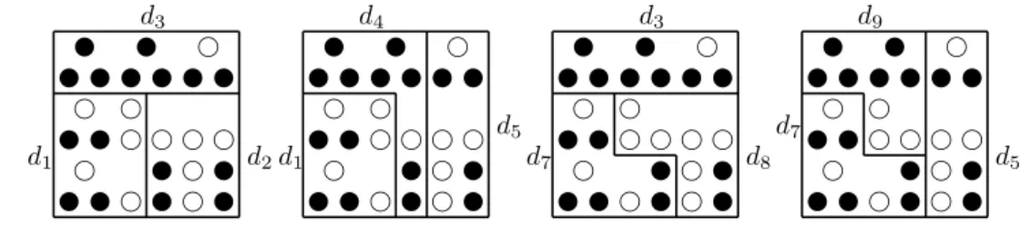
By contrast, the other solutions considered in Section 2 violate consistency. This can be verified by considering the districting problem Π with t = 3 shown in Fig- ure 1. It consists of 27 voters of which 11 are supporters of party A (indicated by empty circles) and 16 are supporters of partyB (indicated by solid circles), and four admissible districtings D1 = {d1, d2, d3}, D2 = {d1, d4, d5}, D3 = {d3, d7, d8} and D4={d5, d7, d9}. Note that partyAwins two out of the three districts inD1 andD2, respectively, and one of the three districts in D3 and D4, respectively. Consider the solutionME first. Since the difference in the number of winning districts for the two parties is one in all cases, we haveMEΠ={D1, D2, D3, D4}. Consider the districting D₁ ∈ME_Π and Y =d₁∪d₂. Consistency would require that the districting{d1, d₂} is among the chosen districtings if the solution is applied to the restricted problem on Y. But obviously, we have ME_Π|_Y = {{d7, d₈}}, because the districting {d7, d₈} induces a draw between the winning districts onY while the districting{d₁, d₂}entails two winning districts for partyA (and zero districts won by partyB). Similarly,MU violates consistency withD₃ ∈MU_Π and Y =d₇∪d₈ sinceMU_Π={D₁, D₂, D₃, D₄} andMU_Π|_Y ={{d1, d2}}.

v v f v f vf v f v v vf f f f

ff

v v v v v vv v f

d1 d2

d3

ff

v v v v v vv v f d1

d5

d4

ff

v v v v v vv v f

d7 d8

d3

ff

v v v v v vv v f d7

d5

d9

Figure 1: ME, MU andLB violate consistency

To verify, finally, that alsoLBviolates consistency observe first thatLB_Π={D₃, D₄} in Figure 1. ConsiderD₄∈LB_Π andY =d₇∪d₉. Consistency would require that the districting{d7, d9} is among the districtings chosen by the solution on the restricted problem on Y. But it is easily seen that LB_Π|_Y = {{d1, d4}}, since the districting

(8)

{d1, d4} gives rise to a draw between the parties on Y which is closer to their respective relative shares of votes on Y. Thus the least biased solution also violates consistency.

Our final axiom expresses a fundamental principle of fairness in our context, namely the symmetric treatment of partiesex ante.

Axiom 5 (Neutrality). A solution F satisfies neutrality if for any districting problem Π = (X,A, µ, µ_A, µ_B, t, G) and any D ∈ F_(X,A,µ,µ_A_,µ_B_,t,G) it follows that D ∈ F_(X,A,µ,µ_B_,µ_A_,t,G).

It is easily seen that all solutions presented so far with exception of the optimal solution(s) satisfy the neutrality axiom.

In the following we will show that for a large class of geographies no solution can satisfy all five axioms simultaneously. While we consider the neutrality condition to be an indispensable fairness requirement, our proof strategy is to show that the first four axioms characterize the optimal partisan gerrymandering solution O. Since this solution evidently violates the neutrality requirement the impossibility result follows.

5 A Characterization Result and an Impossibility

First, we consider districting problems with only two districts.

Lemma 1. F satisfies two-district determinacy, two-district uniformity and indifference if and only ifF =O,F =ME orF =MU fort= 2.

Proof. Observe that two-district determinacy and two-district uniformity reduces the number of possible districting rules for t = 2 to O, ME and MU if only the number of winning districts matters (recall thatME =LB on all two-district problems).

Now indifference ensures that either alltwo-to-zero, all one-to-one, or allzero-to-two districtings admissible for problem Π have to be selected by solutionF.

Finally, we have seen that O, ME and MU satisfy two-district determinacy, two- district uniformity and indifference, which completes the proof.

Consider districting problems for t = 3 with the 9 possible districts and the 3 resulting districtings shown in Figure 2, in which party A voters are indicated by empty circles and party B voters by solid circles, µ equals the counting measure on (X,A) andµA, µB determine the respective number of party A and partyB voters.

It can be verified that, considering the districtings from left to right, we obtain 3 to 0, 2 to 1 and 1 to 2 winning districtings for partyA, respectively. Thus, e.g. the optimal solution for party A would choose the first districting from the left, while the least biased solution would choose the middle districting. The geography in the depicted problem is “thin” in the sense that all proper subproblems allow only one possible districting. Therefore, the consistency condition has no bite at all in this problem. In order to make use of the consistency property, we will restrict the family of admissible geographies in the following way.

Definition 9. The geography Gof a problem Π = (X,A, µ, µA, µB, t, G) islinked if for any two possible districtings D, D⁰ ∈ DΠ there exists a sequence D1, . . . , Dk of districtings such thatD=D1,D⁰ =Dkand #Di∩Di+1=t−2 for alli= 1, . . . , k−1.

(9)

d d t t d t d d d t t d d d d t t t d d d d t t d d t t d t d d d t t d

@

@@

@

@@ d d t t d t d d d t t d d d d t t t d d d d t t d d t t d t d d d t t d

d d t t d t d d d t t d d d d t t t d d d d t t d d t t d t d d d t t d

Figure 2: Unlinked districtings

In the appendix, we present a large and natural class of linked geographies. While the linkedness condition clearly limits the scope of our analysis, there is no hope to obtain characterization results of the sort derived here without further assumptions on the family of geographies.

Proposition 1. If F equals O^A for t = 2 and F is consistent and indifferent, then F =O^A for linked geographies.

Proof. Consider a districting problem Π = (X,A, µ, µA, µ_B, t, G) witht≥3 and suppose that F_Π 6= OÂ_Π but F is consistent and indifferent. Since F_Π is not O_ΠÂ, there exist D⁰ ∈ O_ΠÂ and D ∈ F_Π such that δ_A(D⁰) > δ_A(D) by indifference. Since Π has a linked geography there exists a sequence D₁, . . . , D_k of districtings such that D⁰ = D1, D = Dk and #Di ∩Di+1 = t −2 for all i = 1, . . . , k −1. Let i⁰ = max{i ∈ {1, . . . , k−1} : δA(D1) = δA(D2) = . . . = δA(Di) > δA(Di+1)} and j⁰ = min{j ∈ {2, . . . , k}:δA(D_j−1)6=δA(Dj) =. . .=δA(Dk)}. It follows by indifference thatDi⁰ ∈OÂ_Π andDj⁰ ∈FΠ.

Ifi⁰=j⁰−1, thenDi⁰ andDj⁰ just differ in two districts, which we shall denote by d,d⁰, eande⁰, where the first two districts belong toDi⁰ while the latter two to Dj⁰. Observe thatDi⁰\ {d, d⁰}=Dj⁰\ {e, e⁰} by linkedness. LetY =d∪d⁰ =e∪e⁰. Since O^A andF are consistent we have{d, d⁰} ∈O_Π|^A

Y and{e, e⁰} ∈F_Π|_Y. Our assumption thatF equalsO^Afort= 2 andD_i⁰\ {d, d⁰}=D_j⁰\ {e, e⁰}impliesδ_A(D_i⁰) =δ_A(D_j⁰);

a contradiction.

Assume thati⁰ < j⁰−1. Employing (1), consistency and linkedness, we have

|δA(Di)−δA(Di+1)| ≤1 (5) for alli=i⁰, . . . , j⁰−1 becauseDi andDi+1 just differ in two districts. Moreover, by the definition ofj⁰, by consistency and by our assumption thatFequalsO^Afort= 2 we must haveδA(Dj⁰−1)< δA(Dj⁰), which in turn implies by (5) andδA(Di⁰)> δA(Dj⁰−1) that there exists a smallestj^∗∈ {i⁰+ 1, . . . , j⁰} such thatδA(Dj^∗) =δA(Dj⁰). Clearly, D_j∗∈F_Π by indifference. We cannot have j^∗> i⁰+ 1 since this would contradict the definition of j^∗, D_j^∗ ∈ F_Π, δ_A(D_j^∗₋₁) < δ_A(D_j^∗) and (5). However, if i⁰ = j^∗−1, then we can repeat the argument of the previous paragraph by replacingj⁰ withj^∗to obtain a contradiction.

Since neither the most equal or most unequal solutions satisfy consistency we cannot extendME orMU fort= 2 to arbitrary t in a manner of Proposition 1. However, it might be the case that ME or MU for t = 2 can be extended to another consistent solution. The next proposition demonstrates that such an extension does not exist.

(10)

Proposition 2. There does not exist a consistent and indifferent solutionF that equals ME orMU fort= 2 even for linked geographies.

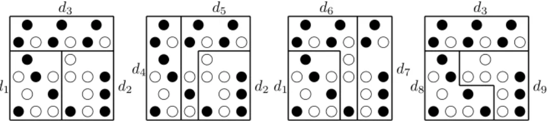
Proof. Suppose that there exists a consistent and indifferent solution F that equals ME fort= 2. Consider the districting problem Π = (X,A, µ, µA, µ_B,3, G), whereX consists of 27 voters,Aequals the set of all subsets ofX, µis the counting measure, andG={d₁, . . . , d₉}is as shown in Figure 3 in which partyAsupporters are indicated by empty circles and partyB supporters by solid circles.

v f f v f vf f v f vv v f f v

f f v f v f v fv v v

d1 d2

d₃

f f v f v f v fv v v d4

d2

d₅

f f v f v f v fv v v d1

d7

d₆

f f v f v f v fv v v

d8 d9

d₃

Figure 3: MEandMU cannot be extended

We can see from Figure 3 that the four possible districtings are D₁ ={d1, d₂, d₃}, D₂ ={d₂, d₄, d₅}, D₃={d₁, d₆, d₇} andD₄={d₃, d₈, d₉}. It can be checked that the given geography is linked. Since δ_A(D₁) = 2 and δ_A(D₂) = δ_A(D₃) = δ_A(D₄) = 1 we must have either {D1} = FΠ, {D2, D3, D4} = FΠ or {D1, D2, D3, D4} = FΠ by indifference. First, consider the cases of {D1} = FΠ and {D1, D2, D3, D4} = FΠ. By consistency we must have {d1, d2} ∈ F_(X⁰_,A⁰_,µ⁰_,µ⁰

A,µ⁰_B,2,G⁰), where X⁰ = d1 ∪d2, G⁰ = {d1, d2, d8, d9} and A⁰, µ⁰, µ⁰_A, µ⁰_B denote the restrictions of A, µ, µA, µB to X⁰, respectively. However, F_(X⁰_,A⁰_,µ⁰_,µ⁰

A,µ⁰_B,2,G⁰) should equal {d8, d9} since F =ME for t= 2; a contradiction. Second, consider the case of {D2, D3, D4}=FΠ and pick the case of D3. By consistency we must have{d6, d7} ∈F_(X⁰⁰_,A⁰⁰_,µ⁰⁰_,µ⁰⁰

A,µ⁰⁰_B,2,G⁰⁰), where X⁰⁰=d6∪d7,G⁰⁰ ={d2, d3, d6, d7} and A⁰⁰, µ⁰⁰,µ⁰⁰_A, µ⁰⁰_B denote the restrictions of A, µ, µA, µB toX⁰⁰, respectively. However, F(X⁰⁰,A⁰⁰,µ⁰⁰,µ⁰⁰_A,µ⁰⁰_B,2,G⁰⁰)should equal {d2, d3} sinceF=ME fort= 2; a contradiction.

Now suppose that there exists a consistent and indifferent solution F that equals MU for t = 2. Consider once again the problem shown in Figure 3. First, consider the cases of {D1} =F_Π and {D1, D₂, D₃, D₄} = F_Π. By consistency we must have {d₁, d₃} ∈ F_(X0,A⁰,µ⁰,µ⁰_A,µ⁰_B,2,G⁰), where X⁰ = d₁∪d₃, G⁰ = {d₁, d₃, d₄, d₅} and A⁰, µ⁰, µ⁰_A, µ⁰_B denote the restrictions of A, µ, µ_A, µ_B to X⁰, respectively. How- ever, F_(X0,A⁰,µ⁰,µ⁰_A,µ⁰_B,2,G⁰) should equal {d4, d5} since F = MU for t = 2; a contradiction. Second, consider the case of {D2, D3, D4} = FΠ and pick the case of D4. By consistency we must have {d8, d9} ∈F_(X⁰⁰_,A⁰⁰_,µ⁰⁰_,µ⁰⁰

A,µ⁰⁰_B,2,G⁰⁰), where X⁰⁰=d8∪d9, G⁰⁰ ={d1, d2, d8, d9} and A⁰⁰, µ⁰⁰, µ⁰⁰_A, µ⁰⁰_B denote the restrictions of A, µ, µA, µB to X⁰⁰, respectively. However,F_(X⁰⁰_,A⁰⁰_,µ⁰⁰_,µ⁰⁰

A,µ⁰⁰_B,2,G⁰⁰)should equal{d1, d2}sinceF=MU fort= 2; a contradiction.

Our main theorem follows from Lemma 1 and Propositions 1 and 2.

Theorem 1. The optimal solutionO is the only solution that satisfies two-district determinacy, two-district uniformity, indifference and consistency on linked geographies.

We obtain the following result as a simple corollary.

(11)

Corollary 1. There does not exist a two-district determinate, two-district uniform, indifferent, consistent and neutral solution on linked geographies.

Appendix

We provide an example showing that linkedness is satisfied by a quite natural planar geography. A bounded subsetAofR² will be calledstrictly connected if its boundary

∂A is a Jordan curve. A subsetA of a strictly connected set B ⊆R² separates B if B\A is not strictly connected. We call a continuous function f : X → R nowhere constant if for anyx∈ X and any neighborhood N(x) of xthere exists a y ∈ N(x) such thatf(x)6=f(y).

Example 1 (Regular). A districting problem Π = (X,B(X), µ, µ_A, µ_B, t, G) is called regular if

1. X is a bounded and strictly connected subset ofR²,

2. µ, µA and µB are finite and absolutely continuous measures on (X,B(X)) with respect to the Lebesgue measure,

3. G consists of all bounded, strictly connected and µ(X)/tsized subsets of B(X) and

4. there exists a continuous nowhere constant function f : X → R such that µA(C) =R

Cf(ω)dµ(ω) for allC∈ B(X).

The last assumption is a purely technical one providing a sufficient condition to ensure that the districtings emerging in the proof of Lemma 2 can be selected in a way that they satisfy (1).

In what follows we write D ∼D⁰ if for two districtingsD, D⁰ ∈ D_Π there exists a sequenceD₁, . . . , D_k of districtings such thatD=D₁,D⁰ =D_kand #D_i∩D_i+1=t−2 for alli= 1, . . . , k−1.

Lemma 2. Regular districting problems are linked.

Proof. Linkedness is clearly satisfied ift= 1 ort= 2. We show that the linkedness of all regular districting problems fort≤nimplies the linkedness of all regular districting problems fort=n+ 1, which yields by induction the proof of our statement.

Take two arbitrary districtings D and E of a districting problem with t =n+ 1.

We can pick a districtd∈Dsuch thatdandX have at least a non-degenerate curve as a common boundary andddoes not separateX, i.e. there exists a curveCof positive length such thatC⊆∂d∩∂X andX\dremains strictly connected. Moreover, there exist a districte∈E and a curveC⊂R² of positive length such thatµ(d∩e)>0 and C⊆∂d∩∂e∩∂X.

Case 1: Assume that e does not separate X. Since µ is absolutely continuous there exists a seth such that µ(h) = 2µ(X)/(n+ 1), d∪e⊂h, d⁰ =h\d ∈G and e⁰ =h\e∈Gand hdoes not separate X. Let H be a districting ofY =X\hinto n−1 strictly connected districts. Then Π |Y∪d⁰ and Π |Y∪e⁰ are regular districting problems, and therefore it follows by the induction hypothesis that D ∼ H∪ {d, d⁰} andH∪ {e, e⁰} ∼E. Clearly{d, d⁰} ∼ {e, e⁰}, which givesH∪ {d, d⁰} ∼H∪ {e, e⁰}.

(12)

Case 2: Assume thatedoes separateX, where the number of strictly disconnected regions of X \ {e} equals k ≤ n. Then d^c∩∂e∩∂X 6= ∅. We can find a district e⁰ ∈ E with a unique boundary element x ∈ ∂e⁰ satisfying x ∈ d^c∩∂e∩∂X and that ∂e∩∂e⁰ has a common curve of positive length starting fromx. Hence, one can exchange territories between eand e⁰ so that for the resulting new districtshand h⁰ we have thatd∩e⊂h,hseparatesX into at mostk−1 strictly disconnected regions.

Clearly, E⁰ = (E\ {e, e⁰})∪ {h, h⁰} ∼ E and we can continue with either Case 1 or Case 2, where nowE⁰ and hplays the role ofE and e, respectively. Observe that we arrive to Case 1 after at mostksteps.

References

[1] Balinski, M.and Young, H.P. (2001),Fair Representation. Meeting the Ideal of One Man, One Vote, Second Edition, Brookings Institution Press, Washington D.C.

[2] Besley, T.andPreston, I.(2007), “Electoral Bias and Public Choice: Theory and Evidence,”Quarterly Journal of Economics122, 1473-1510.

[3] Chambers, P.C. (2008), “Consistent Representative Democracy,” Games and Economic Behavior62, 348-363.

[4] Chambers, P.C. (2009), “An Axiomatic Theory of Political Representation,”

Journal of Economic Theory, 144, 375-389.

[5] Coate, S.andKnight, B.(2007), “Socially Optimal Districting: A Theoretical and Empirical Exploration,”Quarterly Journal of Economics122, 1409-1471.

[6] Friedman, J.N.and Holden, R.T.(2008), “Optimal Gerrymandering: Some- times Pack, But Never Crack,”American Economic Review, 98, 113-144.

[7] Gul, R. and Pesendorfer, W. (2009), “Strategic Redistricting,” American Economic Review, forthcoming.

[8] Puppe, C. and Tasn´adi, A.(2008), “A Computational Approach to Unbiased Districting,”Mathematical and Computer Modelling48, 1455-1460.