Axiomatic districting

Axiomatic Districting by

Clemens Puppe Attila Tasnadi

C O R VI N U S E C O N O M IC S W O R K IN G P A PE R S

http://unipub.lib.uni-corvinus.hu/1464

CEWP 1/2014

Axiomatic districting ^∗

Clemens Puppe

Department of Economics, Karlsruhe Institute of Technology^†

and Attila Tasn´ adi

MTA-BCE “Lend¨ulet” Strategic Interactions Research Group, Department of Mathematics, Corvinus University of Budapest^‡

September 16, 2013

Abstract

In a framework with two parties, deterministic voter preferences and a type of geographical constraints, we propose a set of simple axioms and show that they jointly characterize the districting rule that maximizes the number of districts one party can win, given the distribution of individual votes (the “optimal ger- rymandering rule”). As a corollary, we obtain that no districting rule can satisfy our axioms and treat parties symmetrically.

JEL Classification Number: D72 Keywords: districting, gerrymandering.

1 Introduction

The districting problem has received considerable attention recently, both from the political science and the economics viewpoint.¹ Much of the recent work has focused on strategic aspects and the incentives induced by different institutional designs on the political parties, legislators and voters (see, among others, Besley and Preston, 2007, Friedman and Holden, 2008, Gul and Pesendorfer, 2010). Other contributions have looked at the welfare implications of different redistricting policies (e.g. Coate and Knight, 2007). Finally, there is also a sizable literature on the computational aspects of the districting problem (see, e.g. Puppe and Tasn´adi, 2008, and the references therein, and Ricca, Scozzari and Simeone, 2011, for a general overview of the operations research literature on the districting problem).

∗We are most grateful to an editor and two anonymous referees for their thorough remarks and suggestions which helped to improve the first version of this paper.

†D – 76131 Karlsruhe, Germany, clemens.puppe@kit.edu

‡H – 1093 Budapest, F˝ov´am t´er 8, Hungary, attila.tasnadi@uni-corvinus.hu

1See, e.g., Tasn´adi (2011) for an overview.

In contrast to these contributions, the present paper takes a normative point of view. We formulate desirable properties (“axioms”), and investigate which district- ing rules satisfy them. The axiomatic method allows one to endow the vast space of conceivable districting rules with useful additional structure: each combination of de- sirable properties characterizes a specific class of districting rules, and thereby helps one to assess their respective merits. Furthermore, one may hope that specific combi- nations of axioms single out a few, perhaps sometimes even a unique districting rule, thus reducing the space of possibilities. Finally, the axiomatic approach may reveal incompatibility of certain axioms by showing thatnodistricting rule can satisfy certain combinations of desirable properties, thereby terminating a futile search.

In a framework with two parties and geographical constraints on the shape of dis- tricts, we propose a set of five simple axioms which are motivated by considerations of fairness to voters. The first three axioms restrict the informational basis needed for the construction of a districting. Essentially, they jointly amount to the requirement that the only information that may enter a fair districting rule is thenumber of dis- tricts won by the parties. The motivation for such a requirement is that, ultimately, voters care only about outcomes, i.e. the implemented policies, but these outcomes only depend on the distribution of seats in the parliament – through some political decision process that is not explicitly modeled here. Thus, for instance, if two different districtings induce the same seat shares in the parliament, then either none or both should be considered fair since they are indistinguishable in terms of final outcomes.

Restricting the informational basis for the assessment of districting rules to the pos- sible seat distributions they imply is also attractive from the viewpoint of managing the complexity of the districting problem, since evidently it greatly simplifies the is- sue. Our approach is thus “consequentialist” in the sense that the relative merits of a districting are measured only by the possible outcomes it produces. The destricting process as such does not matter. We emphasize that the geographical constraints nev- ertheless play an important role: they enterindirectly in the assessment of districtings since they influence the possible numbers of districts each party can win. For instance, a bias in the seat share in favor of one party may be acceptable if it is forced by the given geographical constraints, but not if it is avoidable by an alternative admissible districting.

Our fourth condition, the “consistency axiom,” requires that an admissible dis- tricting should induce admissible sub-districtings on any appropriate subregion. This axiom reflects the normative principle that a “fair” institution must be fair in every part (cf. Balinski and Young’s uniformity principle, 2001), or more concretely in our context: a representation of voters via a districting is globally fair only if it is also locally fair. The consistency condition greatly simplifies the internal structure of the admissible districtings, too. The fifth and final condition requires anonymity, i.e. that the districting should be invariant with respect to a re-labeling of parties. In our context, such anonymity requirement has a straightforward normative interpretation in terms of fairness since it amounts to an equal treatment of parties (and voters) ex-ante.

An important conceptual ingredient (and mathematical challenge) of our analysis is the presence of geographical constraints. We model this via an exogenously given collection ofadmissibledistricts from which a districting selects a subset that forms a partition of the entire region. We impose one restriction on the collection of admissible districts other than the standard requirement of equal population mass: that it be

possible to move from one admissible districting to any other admissible districting via a sequence of intermediate districtings changing only two districts at each step.² This

“linkedness”condition is satisfied by a large class of geographies. Except for a technical

“no-ties” assumption, no other restriction is imposed on the collection of admissible districts, thus our approach is very general in this respect. In particular, theabsenceof geographical constraints can be modeled by takingall subregions of equal population mass as the collection of admissible districts (which gives rise to a linked geography).

Moreover, restrictions that are frequently imposed on the shape of districts in practice, such as compactness or contiguity, can in principle be incorporated in our approach by an appropriate choice of admissible districts; for an explicit analysis of these and related issues, see e.g. Chambers and Miller (2010, 2013) and the references given there.

We prove that on all linked geographies, the first four of our axioms jointly charac- terize the districting rule which maximizes the number of districts thatone party can win, given the distribution of individual votes (the “optimal gerrymandering rule”).

Evidently, by generating a maximal number of winning districts for one of the two parties, the optimal gerrymandering rule violates the anonymity condition. As a corol- lary, we therefore obtain that no districting rule can satisfy all five axioms. The result also suggests that any reasonable districting rule must necessarily be complex: either it has a complex internal structure by violating the consistency principle, or it has to employ a complex informational basis in the sense that it depends on more than the merenumber of districts won by each party.

The work closest to ours in the literature is Chambers (2008, 2009) who also takes an axiomatic approach. However, one of his central conditions is the requirement that the election outcome beindependentof the way districts are formed (“gerrymandering- proofness”), and the main purpose of his analysis is to explore the consequences of this requirement (for a similar approach, see Bervoets and Merlin, 2011). By contrast, our focus is precisely on the issue how the districting influences the election outcome, and the aim of our analysis is to structure the vast space of possibilities by means of simple principles. In particular, geographical constraints which are absent in Chambers’ model play an important role in our analysis.

The paper by Landau, Reid and Yershov (2009) also addresses the issue of “fair”

districting. However, unlike our work their paper is concerned with the question of how toimplementa fair solution to the districting problem by letting the parties themselves determine the boundaries of districts. Specifically, these authors propose a protocol similar in spirit to the well-known divide-and-choose procedure.

The districting rules that we consider depend among other things on the distribution of votes for each party in the population. One might argue, perhaps on grounds of some “absolute” notion ofex ante fairness, that a districting rule must not depend on voters’ party preferences since these can change over time. From this perspective, the districting problem is not really an issue and it would seem that any districting which partitions the population in (roughly) equally sized subgroups should be acceptable. By contrast, in the present paper we are interested in a “relative” orex post notion of fair districting, i.e. in the question of what would constitute an acceptable districting rule giventhe distribution of the supporters of each party in the population. This question seems particularly important for practical purposes since a districting policy can be successfully implemented only if it receives sufficient support by theactual legislative

2Since a districting forms a partition of the given region, it is evidently not possible to move from one districting to another districting by changing onlyonedistrict.

body.

2 The Framework

We assume that parties A and B compete in an electoral system consisting only of single member districts, where the representatives of each district are determined by plurality. The parties as well as the independent bodies face the following districting problem.

Definition 1 (Districting problem). A districting problem is given by the structure Π = (X,A, µ, µA, µ_B, t, G), where

• the voters are located within a subset X of the planeR²,

• A is the σ-algebra on X consisting of all districts that can be formed without geographical or any other type of constraints,

• the distribution of voters is given by a measureµon (X,A),

• the distributions of party A and partyB supporters are given by measures µA

andµB on (X,A) such thatµ=µA+µB,

• t is the given number of seats in parliament,

• G ⊆ A, also called geography, is a collection of admissible districts satisfying µ(g) =µ(X)/tand

µ_A(g)6=µ_B(g) (1)

for allg∈G, and admitting a partitioning ofX, i.e there exist mutually disjoint sets g⁰₁, . . . , g⁰_t∈Gsuch that∪^t_i=1g_i⁰=X.

Condition (1) excludes ties in the distribution of party supporters in all admissible districts to avoid the necessity of introducing tie-breaking rules. This condition is satisfied, for instance, if the set of voters is finite,µ, µA, µB are the counting measures and the district sizes are odd.

Definition 2(Districting). Adistricting for problem Π = (X,A, µ, µA, µB, t, G) is a subsetD⊆Gsuch thatD forms a partition ofX and #D=t.

We shall denote byδA(D) and δB(D) the number of districts won by partyA and partyB under D, respectively. We write DΠfor the set of all districtings of problem Π and letδA(D) ={δA(D) :D∈ D}andδB(D) ={δB(D) :D∈ D}for anyD ⊆ DΠ. Definition 3 (Solution). A solution F associates to each districting problem Π a non-empty set of chosen districtingsF_Π⊆ DΠ.

3 Several Solutions

We now present a number of simple solution candidates. The first solution determines the optimal partisan gerrymandering from the viewpoint of partyA.

Definition 4 (Optimal solution for A). The optimal solutionO^A for party Adeter- mines for districting problem Π = (X,A, µ, µA, µB, t, G) the set of those districtings that maximize the number of winning districts for partyA, i.e.

O_Π^A= arg max

D∈DΠ

δ_A(D).

Evidently, in the absence of other objectives, O^A is the solution favored by party A supporters. The optimal solutionO^B for party B is defined analogously. If we are referring to an optimal solutionO, then we have eitherO^A orO^B in mind.

The next solution minimizes the difference in the number of districts won by the two parties. It has an obvious egalitarian spirit.

Definition 5(Most equal solution). The solutionMEdetermines for districting prob- lem Π = (X,A, µ, µA, µB, t, G) the set of most equal districtings, i.e.

ME_Π= arg min

D∈DΠ

|δA(D)−δ_B(D)|. (2) Clearly, depending on the distribution of votes in the population, an equal distri- bution of seats in the parliament may not be possible. The most equal solution aims to get as close as possible to equality in terms of the number of winning districts for the two parties.

The third solution maximizes the difference in the number of districts won by the two parties. The objective to maximize the winning margin of the ruling party could be motivated, for instance, by the desire to avoid too much political compromise.

Definition 6 (Most unequal solution). The solution MU determines for districting problem Π = (X,A, µ, µ_A, µ_B, t, G) the set of most unequal districtings, i.e.

MU_Π= arg max

D∈D_Π|δ_A(D)−δ_B(D)|. (3) Fourth, we consider the solution that minimizes partisan bias. It has a clear mo- tivation from the point of view of maximizing representation of the “people’s will” in the sense that the share of the districts won by each party is as close as possible to its share of votes in the population.

Definition 7(Least biased solution). The solutionLBdetermines for districting prob- lem Π = (X,A, µ, µ_A, µ_B, t, G) the set of those districtings that minimize the absolute difference between shares in winning districts and shares in votes, i.e.

LB_Π= arg min

D∈D_Π

δA(D)

t −µA(X) µ(X)

= arg min

D∈D_Π

δB(D)

t −µB(X) µ(X)

. (4)

Finally, we mention the trivial solution that associates to each problem the set of alladmissible districtings.

Definition 8 (Complete solution). The complete solutionC associates with any dis- tricting problem Π = (X,A, µ, µA, µB, t, G) the set of all possible districtingsDΠ.

4 Axioms

In this section, we formulate five simple axioms and argue that each has appeal from a normative (and sometimes also from a pragmatic) point of view.

The case of two districts plays a fundamental role in our analysis. Note that by (1) it is not possible that a party can win both districts under one districting and lose both districts under another districting, i.e. if t = 2 then δA(DΠ) (respectively, δB(DΠ)) cannot contain both 0 and 2. Our first axiom requires that a solution must in fact be “determinate” in the two-district case in the sense that it must not leave open the issue whether there is a draw between the two parties or a victory for one party.

In other words, if a solution chooses a districting that results in a draw between the parties for a given problem it cannot choose another districtingfor the sameproblem that results in a victory for one party.

Axiom 1 (Two-district determinacy). A solutionF satisfiestwo-district determinacy if for any districting problem Π witht= 2, the setsδA(FΠ) andδB(FΠ) are singletons.³ The motivation for this axiom stems from our implicit assumption that voters do not care about the districtings as such, but only about the entailed shares of seats in the parliament, since it is the latter that influences final outcomes. Any indeterminacy in the distribution of seats in the parliament potentially influences the outcome and would thus introduce an element of arbitrariness of the final state of affairs. In the two-district case, such indeterminacy necessarily turns a (unanimous) victory of one party into a draw between the two parties, or vice versa. Two-district determinacy prevents this to occur.

Evidently, all solutions considered in Section 2 with the exception of the complete solutionCsatisfy Axiom 1. Also observe that on the family of all two-district problems the most equal solutionME and the least biased solutionLB coincide.⁴

Our next axiom requires that a solution behaves “uniformly” on the set of two- district problems in the sense that the solution must treat different two-district prob- lems in the same way, provided they admit the same set of possible distributions of the number of districts won by each party.

Axiom 2 (Two-district uniformity). A solution F satisfiestwo-district uniformity if for any districting problems Π and Π⁰ with t= 2 such that δ_A(DΠ) =δ_A(DΠ⁰) (and therefore also δ_B(D_Π) = δ_B(D_Π⁰)) we have δ_A(F_Π) = δ_A(F_Π⁰) (and therefore also δ_B(F_Π) =δ_B(F_Π⁰)).

Even though it is imposed only in the two-district case, Axiom 2 is admittedly a strong requirement. It can be motivated by invoking again the assumption that vot- ers care about districtings only via their influence on political outcomes. From this perspective, Axioms 2 states that if the possible political outcomes are the same in different two-district problems, then the actual outcome should also be the same. A violation of Axiom 2 would mean that characteristics other than the possible distri- butions of seat shares can influence the solution and hence the final outcome. But if

3Observe that overall determinacy, i.e. thatδA(FΠ) andδB(FΠ) be singletons foreveryproblem Π, is a strictly stronger requirement than two-district determinacy; for instance, the least biased solution satisfies two-district determinacy but can easily be shown to violate overall determinacy.

4To verify this, observe that if there exist admissible districtingsD, D⁰∈ DΠwithδA(D) = 2 and δA(D⁰) = 1, then one must have 0.5< µA(X)/µ(X)<0.75. Thus,D⁰must be chosen both byME andLB.

these characteristics play no role in voters’ preferences, it is not clear how one could justify such influence. To illustrate, consider two districting problems Π and Π⁰ with δA(DΠ) = δA(DΠ⁰) = {1,2}; thus, in either situation there exists one districting un- der which partyA wins both districts and another districting which produces a draw between the two parties. Now assume that party A’s share of votes in situation Π is in fact larger than its share of votes in situation Π⁰, i.e.µ_A> µ⁰_A. Couldn’t this give a good reason to select the districting under which A wins both seats in situation Π but the districting in which both parties receive one seat in situation Π⁰, provided that the difference between µA and µ⁰_A is sufficiently large? But then, how large precisely is “sufficiently large”? Is x% enough? And wouldn’t the threshold also have to de- pend on the absolute level ofµA? Two-district uniformity answers these question by a very clearcut and simple recommendation: different treatment of different two-district situations, for instance on the grounds that one party has a larger share of votes in one of the situations, is justified only if the difference manifests itself in a difference of the possible number of seats in parliament that the parties can win. Two-district uniformity thus sets a high “threshold” for differential treatment of two-district situa- tions. We emphasize therefore that all candidate solutions presented in Section 2 above satisfy this condition; for the least biased solution this follows from Footnote 4, for the other solutions it is evident.

A secondary motivation for Axiom 2 is to keep the complexity of a districting solution manageable. Indeed, any influence of characteristics different from the possible seat distribution in parliament – whether derived from the underlying distribution of party supporters or from geographical information – would considerably complicate the definition and implementation of a districting rule.

Our third axiom, imposed on districting problems of any size, has a motivation related to that of the two previous axioms. It states that if a possible districting induces the same distribution of the number of winning districts for each party than some districting chosen by a solution, it must be chosen by this solution as well.

Axiom 3(Indifference). A solutionF satisfiesindifference if for any districting prob- lem Π we have that D∈FΠ,D⁰ ∈ DΠ, δA(D) =δA(D⁰) andδB(D) =δB(D⁰) implies D⁰∈FΠ.

The justification of the indifference axiom is straightforward under the intended notion of fairness to voters. If voters care only about final outcomes, and if final outcomes only depend on seat shares, then two districtings that entail the same seat distribution in parliament are undistinguishable in terms of final outcomes and have therefore to be treated equally. Evidently, all solutions presented above satisfy this condition.

The following consistency axiom plays a central role in our analysis. It requires that a solution to a problem should also deliver appropriate solutions to specific sub- problems. Its spirit is very similar to theuniformity principle in Balinski and Young’s (2001) theory of apportionment (“every part of a fair division should be fair”).

Prior to the definition of consistency we have to introduce specific subproblems of a districting problem. For any problem Π, any D ∈ FΠ and any D⁰ ⊆ D, let Y =

∪d∈D⁰d and define the subproblem Π|Y to be (Y,A|Y, µ|Y, µA|Y, µB|Y,#D⁰, G|Y), whereA|Y ={A∩Y :A∈ A},G|Y ={g∈G:g⊆Y} andµ|Y, µA|Y, µB|Y stand for the restrictions of measuresµ, µA, µB to (Y,A|Y).

Axiom 4(Consistency). A solutionF satisfiesconsistency if for any districting prob- lem Π, anyD∈FΠ and anyD⁰⊆D we have forY =∪d∈D⁰dthat

D⁰∈F_Π|Y.

The motivation for imposing the consistency condition in our context is as follows.

Most federal countries have both federal and local legislatures, and in many of those countries the same districts are used for both, local and federal elections. The con- sistency axiom requires that a districting is a global solution, i.e. can be considered

“globally fair,” only if it also represents a solution on all appropriate subregions, i.e. is also everywhere “locally fair.”⁵ In other words, consistency forbids to create a globally fair treatment of voters by equilibrating different locally unfair treatments. Moreover, it justifies using the same districts locally and globally – as is common practice in most countries. Finally, consistency may also be of practical value if regions decide to separate, or to increase political independence, since it would allow them to use the same districting as before.

The optimal and complete solutions satisfy consistency. This is evident for the complete solution. To verify it for the optimal solution suppose, by contradiction, that there would existD⁰⊂D∈O^A_Π such thatD⁰∈/O^A_Π|

Y, whereY =∪_d∈D⁰d. This would implyδ_A(D⁰⁰∪(D\D⁰))> δ_A(D) for anyD⁰⁰∈O_Π|^A

Y, a contradiction.

By contrast, the other solutions considered in Section 2 violate consistency. This can be verified by considering the districting problem Π witht= 3 shown in Fig. 1. It consists of 27 voters of which 11 are supporters of partyA(indicated by empty circles) and 16 are supporters of partyB (indicated by solid circles), and four admissible dis- trictingsD1={d1, d2, d3},D2={d1, d4, d5}, D3={d3, d7, d8} andD4={d5, d7, d9}.

Note that partyAwins two out of the three districts inD1and D2, respectively, and one of the three districts inD3 andD4, respectively. Consider the solution ME first.

Since the difference in the number of winning districts for the two parties is one in all cases, we haveMEΠ={D1, D2, D3, D4}. Consider the districtingD1∈MEΠ and Y =d1∪d2. Consistency would require that the districting{d1, d2} is among the cho- sen districtings if the solution is applied to the restricted problem onY. But obviously, we haveME_Π|Y ={{d7, d8}}, because the districting{d7, d8}induces a draw between the winning districts onY while the districting{d1, d2}entails two winning districts for partyA(and zero districts won by party B). Similarly, MU violates consistency with D₃∈MU_Π andY =d₇∪d₈sinceMU_Π={D1, D₂, D₃, D₄}andMU_Π|Y ={{d1, d₂}}.

v v f v f vf v f v v vf f f f

ff

v v v v v vv v f d₁

d₂ d3

v v f v f vf v f v v vf f f f

ff

v v v v v vv v f d₁

d₅ d4

v v f v f vf v f v v vf f f f

ff

v v v v v vv v f

d₇ d₈

d3

v v f v f vf v f v v vf f f f

ff

v v v v v vv v f d₇

d₅ d9

Figure 1: ME,MU andLBviolate consistency.

To verify, finally, that alsoLBviolates consistency observe first thatLB_Π={D3, D₄} in Fig. 1. Consider D₄ ∈LB_Π and Y =d₇∪d₉. Consistency would require that the

5Clearly, this requirement has to be restricted to subregions that areunionsof districts, since a given districting does not necessarily induce an admissible sub-districting on other subregions.

districting{d7, d9} is among the districtings chosen by the solution on the restricted problem on Y. But it is easily seen that LB_Π|Y = {{d1, d4}}, since the districting {d1, d4} gives rise to a draw between the parties on Y which is closer to their re- spective relative shares of votes on Y. Thus the least biased solution also violates consistency.

Our final axiom expresses a very fundamental principle of fairness and equity in our context, namely the symmetric treatment of partiesex ante.

Axiom 5 (Anonymity). A solution F satisfiesanonymity if exchanging the distribu- tions of party A and party B voters µA and µB does not change the set of chosen districtings: for all districting problems Π = (X,A, µ, µA, µB, t, G),

D∈F_{(X,A,µ,µA,µB,t,G)} if and only ifD∈F_{(X,A,µ,µB,µA,t,G)}.

Note that this can also be interpreted as a requirement of anonymity with respect to voters across different parties; indeed, anonymity with respect to voters of the sameparty is already implicit in our definition of a districting problem since only the aggregate mass of parties’ supporters matters and not their identity. It is easily seen that all solutions presented so far with exception of the optimal solution(s) satisfy the anonymity axiom.

In the following we will show that for a large class of geographies no solution can satisfy all five axioms simultaneously. While we consider the anonymity condition to be an indispensable fairness requirement, our proof strategy is to show that the first four axioms characterize the optimal partisan gerrymandering solution O. Since this solution evidently violates anonymity the impossibility result follows.

5 A Characterization Result and an Impossibility

First, we consider districting problems with only two districts.

Lemma 1. F satisfies two-district determinacy, two-district uniformity and indiffer- ence if and only ifF =O,F =ME orF =MU fort= 2.

Proof. Observe that two-district determinacy and two-district uniformity jointly reduce the set of possible districting rules for t = 2 to O, ME and MU if only the number of winning districts matters (recall thatME=LB on all two-district problems). Now indifference ensures that either all two-to-zero, all one-to-one, or all zero-to-two dis- trictings admissible for problem Π have to be selected by solutionF.

Finally, we have seen that O, ME and MU satisfy two-district determinacy, two- district uniformity and indifference, which completes the proof.

Consider a districting problem for t= 3 with the 9 admissible districts and the 3 resulting districtings shown in Fig. 2, in which partyAvoters are indicated by empty circles and partyBvoters by solid circles,µequals the counting measure on (X,A) and µ_A,µ_B are given by the respective number of partyA and partyB voters. It can be verified that, considering the districtings from left to right, we obtain 3 to 0, 2 to 1 and 1 to 2 winning districtings for partyA, respectively. Thus, e.g. the optimal solution for partyAwould choose the first districting from the left, while the least biased solution would choose the middle districting.

d d t t d t d d d t t d d d d t t t d d d d t t d d t t d t d d d t t d

@

@

@@

@

@@ d d t t d t d d d t t d d d d t t t d d d d t t d d t t d t d d d t t d

d d t t d t d d d t t d d d d t t t d d d d t t d d t t d t d d d t t d

Figure 2: Unlinked districtings.

The geography in the depicted problem is “thin” in the sense that all proper sub- problems allow only one possible districting. Therefore, the consistency condition has no bite at all in this problem. In order to make use of the consistency property, we will restrict the family of admissible geographies in the following way.

Definition 9. The geography G of a problem Π = (X,A, µ, µA, µB, t, G) is linked if for any two possible districtings D, D⁰ ∈ DΠ there exists a sequence D₁, . . . , D_k of districtings such thatD=D₁,{D2, . . . , D_k−1} ⊆ DΠ,D⁰ =D_k, and #D_i∩Di+1=t−2 for alli= 1, . . . , k−1.

In the appendix, we present a large and natural class of linked geographies, which arise from what we call regular districting problems. In a regular districting prob- lem, µ is given by some finite measure that is absolutely continuous with respect to the Lebesgue measure, and the admissible districts are the bounded Borel sets whose boundary is a Jordan curve.

While the linkedness condition clearly limits the scope of our analysis, there is no hope in obtaining characterization results of the sort derived here without further assumptions on the family of geographies. Note also that under many specifications of the measure µ the unrestricted geography which admits allsubsets of size µ(X)/t is linked (for instance, this holds if the set of voters is finite and µ is the counting measure).

Proposition 1. If F equals O^A for t = 2 and F is consistent and indifferent, then F =O^A for linked geographies.

Proof. Consider a districting problem Π = (X,A, µ, µA, µB, t, G) witht≥3 and sup- pose that FΠ 6= O^A_Π but F is consistent and indifferent. Since FΠ is not O_Π^A, there exist D⁰ ∈O_Π^A andD ∈FΠ such that δA(D⁰)> δA(D) by indifference. Since Π has a linked geography there exists a sequenceD1, . . . , Dk of districtings such thatD⁰ =D1, {D2, . . . , D_k−1} ⊆ DΠ,D=D_k and #D_i∩D_i+1=t−2 for alli= 1, . . . , k−1.

We claim that

|δA(D_i)−δ_A(D_i+1)| ≤1 (5) for all i = 1, . . . , k−1, where D_i and D_i+1 just differ in two districts. To verify (5) we shall denote the two pairs of different districts by d, d⁰, e and e⁰, where the first two districts belong to D_i while the latter two to D_i+1. Observe that D_i\ {d, d⁰} = D_i+1\ {e, e⁰}by linkedness. Hence,

δA(Di)−δA(Di+1) = δA({d, d⁰}) +δA(Di\ {d, d⁰})−δA({e, e⁰})− δ_A(D_i+1\ {e, e⁰})

= δA({d, d⁰})−δA({e, e⁰}). (6)

By (1) we must have |δA({d, d⁰})−δA({e, e⁰})| ≤ 1, which implies, taking (6) into consideration, (5).

Letj^∗∈ {2, . . . , k} be the smallest index such thatδA(Dj^∗) =δA(Dk). SinceDk ∈ F_Πwe haveD_j^∗∈F_Πby indifference. Linkedness ensures thatD_j^∗₋₁andD_j^∗just differ in two districts, which we shall denote by d, d⁰,e ande⁰, where the first two districts belong toD_j^∗₋₁while the latter two toD_j^∗. Furthermore,D_j^∗₋₁\{d, d⁰}=D_j^∗\{e, e⁰} by linkedness. Let Y =d∪d⁰ =e∪e⁰. Since F is consistent we have {e, e⁰} ∈ F_Π|Y. Our assumption thatF equalsO^Afort= 2 impliesδ_A({d, d⁰})≤δ_A({e, e⁰}). Ifj^∗= 2, by consistency

δA(D1) > δA(Dk) =δA(D2) =δA({e, e⁰}) +δA(D2\ {e, e⁰})

≥ δ_A({d, d⁰}) +δ_A(D₁\ {d, d⁰}) =δ_A(D₁);

a contradiction. Otherwise, suppose thatj^∗>2. Then by consisteny and the optimal- ity of F onY we must haveδ_A(D_j^∗₋₁)≤δ_A(D_j^∗). Moreover, δ_A(D_j^∗₋₁)< δ_A(D_j^∗) by the definition ofj^∗. Then by (5) and

δA(D1)> δA(Dk) =δA(Dj^∗)> δA(Dj^∗−1)

there exists aj⁰ ∈ {2, . . . , j^∗−1} such thatδA(Dj⁰) =δA(Dk). Clearly,Dj⁰ ∈FΠ by indifference, contradicting the definition ofj^∗.⁶

Since neither the most equal or most unequal solutions satisfy consistency we cannot extendME or MU fort= 2 to arbitraryt in the manner of Proposition 1. However, it might be the case thatME or MU for t= 2 can be extended to another consistent solution. The next proposition demonstrates that such an extension does not exist.

Proposition 2. There does not exist a consistent and indifferent solutionF that equals ME orMU fort= 2 even for linked geographies.

Proof. Suppose that there exists a consistent and indifferent solution F that equals ME fort= 2. Consider the districting problem Π = (X,A, µ, µ_A, µ_B,3, G), whereX consists of 27 voters,Aequals the set of all subsets ofX, µis the counting measure, andG={d1, . . . , d9}is as shown in Fig. 3 in which party A supporters are indicated by empty circles and partyB supporters by solid circles.

v f f v f vf f v f vv v f f v

f f v f v f v fv v v

d₁ d₂

d3

v f f v f vf f v f vv v f f v

f f v f v f v fv v v d₄

d₂ d5

v f f v f vf f v f vv v f f v

f f v f v f v fv v v

d₁ d₇

d6

v f f v f vf f v f vv v f f v

f f v f v f v fv v v

d₈ d₉

d3

Figure 3: ME andMU cannot be extended.

We can see from Fig. 3 that the four possible districtings are D1 ={d1, d2, d3}, D2 ={d2, d4, d5}, D3={d1, d6, d7} andD4={d3, d8, d9}. It can be checked that the given geography is linked. Since δA(D1) = 2 and δA(D2) = δA(D3) = δA(D4) = 1

6We would like to thank Dezs˝o Bednay for suggestions that improved our original proof.

we must have either {D1} = FΠ, {D2, D3, D4} = FΠ or {D1, D2, D3, D4} = FΠ by indifference. First, consider the cases of {D1} = FΠ and {D1, D2, D3, D4} = FΠ. By consistency we must have {d1, d2} ∈ F(X⁰,A⁰,µ⁰,µ⁰_A,µ⁰_B,2,G⁰), where X⁰ = d1 ∪d2, G⁰ = {d1, d₂, d₈, d₉} and A⁰, µ⁰, µ⁰_A, µ⁰_B denote the restrictions of A, µ, µ_A, µ_B to X⁰, respectively. However, F_(X0,A⁰,µ⁰,µ⁰_A,µ⁰_B,2,G⁰) should equal {d8, d₉} since F =ME for t= 2; a contradiction. Second, consider the case of {D₂, D₃, D₄}=F_Π and pick the case of D₃. By consistency we must have{d₆, d₇} ∈F_(X00,A⁰⁰,µ⁰⁰,µ⁰⁰_A,µ⁰⁰_B,2,G⁰⁰), where X⁰⁰=d₆∪d₇,G⁰⁰ ={d₂, d₃, d₆, d₇} and A⁰⁰, µ⁰⁰,µ⁰⁰_A, µ⁰⁰_B denote the restrictions of A, µ, µA, µB toX⁰⁰, respectively. However, F_(X00,A⁰⁰,µ⁰⁰,µ⁰⁰_A,µ⁰⁰_B,2,G⁰⁰)should equal {d2, d3} sinceF=ME fort= 2; a contradiction.

Now suppose that there exists a consistent and indifferent solution F that equals MU for t = 2. Consider once again the problem shown in Fig. 3. First, consider the cases of {D1} = FΠ and {D1, D2, D3, D4} = FΠ. By consistency we must have {d1, d3} ∈ F_(X⁰_,A⁰_,µ⁰_,µ⁰

A,µ⁰_B,2,G⁰), where X⁰ = d1∪d3, G⁰ = {d1, d3, d4, d5} and A⁰, µ⁰, µ⁰_A, µ⁰_B denote the restrictions of A, µ, µA, µB to X⁰, respectively. However, F(X⁰,A⁰,µ⁰,µ⁰_A,µ⁰_B,2,G⁰) should equal {d4, d5} since F = MU for t = 2; a contradic- tion. Second, consider the case of {D2, D3, D4} = FΠ and pick the case of D4. By consistency we must have {d8, d9} ∈ F(X⁰⁰,A⁰⁰,µ⁰⁰,µ⁰⁰_A,µ⁰⁰_B,2,G⁰⁰), where X⁰⁰ = d8∪d9, G⁰⁰ ={d1, d₂, d₈, d₉} and A⁰⁰, µ⁰⁰, µ⁰⁰_A, µ⁰⁰_B denote the restrictions of A, µ, µ_A, µ_B to X⁰⁰, respectively. However,F_(X00,A⁰⁰,µ⁰⁰,µ⁰⁰_A,µ⁰⁰_B,2,G⁰⁰)should equal{d1, d₂}sinceF=MU fort= 2; a contradiction.

Our main theorem follows from Lemma 1 and Propositions 1 and 2.

Theorem 1. The optimal solutionO is the only solution that satisfies two-district de- terminacy, two-district uniformity, indifference and consistency on linked geographies.

We verify, on linked geographies, the tightness of Theorem 1, i.e. the independence of the axioms. First, the complete solution only violates two-district determinacy.

Second,ME,MU andLB just violate consistency.

Third, we investigate indifference. Consider the districting problem Π⁰ given by Fig. 4 in whichX⁰ consists of 27 voters,A⁰ equals the set of all subsets ofX⁰,µ⁰ is the counting measure, andG⁰admit the districts shown in Fig. 4, where partyAsupporters are indicated by empty circles and partyB supporters by solid circles. Observe that any two consecutive districtings in the sequenceD₁, . . . , D₄only differ in two districts, and therefore, Π⁰ has a linked geography. We shall denote byF the solution given by

F_Π=







{D₄} if Π = Π⁰,

O^A_Π if Π⁰ is not a subproblem of Π and {D₄} ∪O_Π|^A

X\X0 if Π⁰ is a subproblem of Π,

where the voters of problem Π are located withinXand we say that Π⁰ is a subproblem of Π if Π⁰ = Π|_X⁰ andX⁰can be partitioned into three equally sized districts by picking three districts from the geography of problem Π. It can be verified thatF satisfies two- district determinacy, two-district uniformity and consistency. Clearly,F 6=O^Abecause of δA(D1) = 3 > δA(D4) = 2 and indifference is violated since otherwise D4 ∈ FΠ

should implyD2∈FΠ.

Finally, to verify that two-district uniformity cannot be dropped from the list of conditions in Theorem 1 we are again considering problem Π⁰ from Fig. 4 and are

f f v v f fv v f f f f f fv v f f f f f f v vv Dv1 v

d1

d2

d3

f f v v f fv v f f f f f fv v f f f f f f v vv Dv2 v d4

d5

d3

f f v v f fv v f f f f f fv v f f f f f f v vv Dv3 v

f f v v f fv v f f f f f fv v f f f f f f v vv Dv4 v

Figure 4: Indifference is necessary.

modifying solution F slightly. We shall denote the two-district subproblem of Π⁰ on X1 =X⁰ \ {d3}, which consists in choosing either districting {d1, d2} or {d4, d5}, by Π1. DefineFb as follows,

FbΠ=















{D2, D4} if Π = Π⁰,

O_Π^A if Π⁰ and Π1 are not a subproblems of Π {D2, D4} ∪O^A_Π|

X\X0 if Π⁰ is a subproblem of Π, {{d4, d5}} ∪O_Π|^A

X\X1

if Π⁰ is not a subproblem of Π but Π1is a subproblem of Π.

It can be checked thatFbsatisfies two-district determinacy, indifference and consistency, but violates two-district uniformity.

Remark 1. Two-district determinacy is strictly weaker than overall determinacy⁷ even in the presence of two-district uniformity and consistency.

This can verified by considering the problem Π⁰ defined in Fig. 4 and a slight modification of the construction of solutionFdescribed two paragraphs earlier. Denote byFethe solution given by

Fe_Π=







{D1, D4} if Π = Π⁰,

O^A_Π if Π⁰ is not a subproblem of Π and {D1, D4} ∪O_Π|^A

X\X0 if Π⁰ is a subproblem of Π,

where the voters of problem Π are located within X. It is easily seen that Fe satisfies two-district uniformity, consistency and two-district determinacy, but violates overall determinacy.

We obtain the following result as a simple corollary of Theorem 1.

Corollary 1. There does not exist a two-district determinate, two-district uniform, indifferent, consistent and anonymous solution on linked geographies.

Appendix: Regular Districting Problems

We have already seen examples of linked geographies in Figures 1, 3 and 4. In this ap- pendix we provide a natural and large class of further examples of districting problems with linked geographies.

7For a definition of overall determinacy see Footnote 3.

A bounded subset A of R² will be calledstrictly connected if its boundary ∂A is a Jordan curve (i.e. a non self-intersecting continuous loop). A subsetA of a strictly connected setB⊆R²separatesBifB\Ais not strictly connected. We call a continuous functionf :X→Rnowhere constant if for anyx∈X and any neighborhoodN(x) of xthere exists ay∈N(x) such thatf(x)6=f(y).

Definition 10 (Regular Districting Problems). A districting problem Π = (X,A, µ, µ_A, µ_B, t, G) is calledregular if

1. X is a bounded and strictly connected subset ofR²,

2. Aequals the set of Borel sets onX, i.e. following standard notationA=B(X), 3. µis a finite and absolutely continuous measure on (X,B(X)) with respect to the

Lebesgue measure,

4. G consists of all bounded, strictly connected and µ(X)/tsized subsets lying in B(X) and satisfying (1),

5. there exists a continuous nowhere constant function f : X → R such that µ_A(C) =R

Cf(ω)dµ(ω) for allC∈ B(X), and

6. µ_B is given byµ_B(C) =µ(C)−µ_A(C) for allC∈ B(X).

The fifth condition is a technical assumption to ensure that the districtings emerg- ing in the proof of Lemma 3 below can be selected in a way that they satisfy (1).

Specifically, we have the following lemma.

Lemma 2. If we have two neighboring,⁸ bounded, strictly connected and µ(X)/tsized sets d, e∈ B(X)such that µA(d) = µ(d)/2 (i.e dviolates (1)), then we can exchange territories between dande in a way that the two resulting bounded, strictly connected andµ(X)/tsized sets d⁰, e⁰ ∈ B(X) satisfy (1).

Proof. Pick a pointx∈∂d∩∂efrom the relative interior of the common boundary ofd ande. Sincef is nowhere constant there exists ay arbitrarily close toxin the interior of d such that f(y) 6= f(x). Assume that f(y)> f(x). There exist a neighborhood N_εy(y) ofy and a neighborhood N_εx(x) ofxsuch that

∀z∈Nε_y(y) : f(z)> f(x) +2

3(f(y)−f(x)) and

∀z∈Nε_x(x) : f(z)< f(x) +1

3(f(y)−f(x)) by continuity off.

By establishing a sufficiently thin connection between Nε_y(y) and Nε_x(x), which shall be assigned toe⁰, and exchanging a subset ofNε_y(y) with a subset ofNε_x(x)∩ein a way such thatµ(d) =µ(d⁰) =µ(e) =µ(e⁰), we can guarantee thatµA(d⁰)6=µ(d⁰)/2.⁹

Finally, the case of f(y)< f(x) can be handled in an analogous way.

8We call two subsets of the plane neighboring if they share a common boundary of positive length.

9If µA(e)6=µ(e)/2, thenµA(e⁰)6=µ(e⁰)/2 can be guaranteed by exchanging sets of sufficiently small measureµbetweendande. In addition, ifµA(e) =µ(e)/2 andµA(e⁰) =µ(e⁰)/2, then we can repeat the exchange of territories betweene⁰ andd⁰to ensure that both sets satisfy (1).

In the following, we write D ∼ D⁰ if D, D⁰ ∈ DΠ and there exists a sequence D1, . . . , Dk of districtings such that D = D1, {D2, . . . , Dk−1} ⊆ DΠ, D⁰ = Dk and

#Di∩Di+1=t−2 for alli= 1, . . . , k−1. It is easily verified that∼is an equivalence relation on the set of districtings.

Lemma 3. The geographies of regular districting problems are linked.

Proof. Linkedness is clearly satisfied ift= 1 ort= 2. We show that the linkedness of the geographies of all regular districting problems fort ≤nimplies the linkedness of the geographies of all regular districting problems fort=n+ 1. From this, Lemma 3 follows by induction.

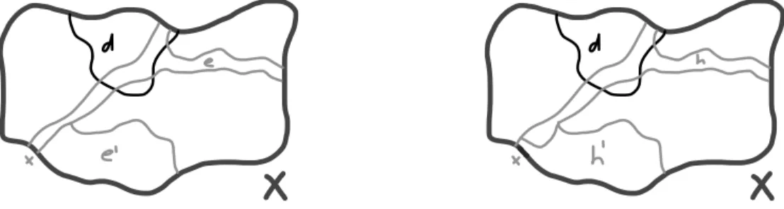
Take two arbitrary districtingsDandEof a districting problem witht=n+ 1. We can pick a districtd∈Dsuch thatdandX have a non-degenerate curve as a common boundary, i.e. there exists a curveC of positive length such thatC ⊆∂d∩∂X. We divide our proof into three steps.

Step 1: We show that there exists a districting D⁰ ∼D that contains a district d⁰ which shares a common boundary of positive length with the boundary of X and which does not separateX.

If d itself does not separate X we are done. Thus, assume that d separates X.

For simplicity, we start with the case in whichdseparatesX into only two regions as shown in the picture on the left of Fig. 5.¹⁰ By exchanging territories between the two

Figure 5: dseparatesX into two regions.

districtsdande, whereeis a neighboring district ofd, as shown in the picture on the left of Fig. 5, we can arrive at districtsd⁰ ande⁰ such thatd⁰ does not separateX.¹¹

More generally, assume that dseparates X, where the number of strictly discon- nected regions of X\ {d} equals k ≤n. We can find a district e∈ D and a unique boundary elementx∈∂esuch thatx∈∂d∩∂Xand such that∂dand∂ehave a common curve of positive length starting fromx. Hence, one can exchange territories betweend andeso that for the resulting new districtsd⁰ ande⁰ we have thatd⁰ separatesX into at most k−1 strictly disconnected regions. Clearly,D⁰ = (D\ {d, e})∪ {d⁰, e⁰} ∼D.

Repeating the described bilateral territorial exchangek−1 times, we thus arrive at a districtingD⁰that contains a districtd⁰ which shares a common boundary withX and which does not separateX.

10Both pictures only show the two districts involved in a territorial exchange and not the entire districtings.

11It might happen thatd⁰ ore⁰ violate (1) since we only took care of the shapes and sizes of the two districts. However, Lemma 2 ensures that through an appropriate territorial exchange between d⁰ande⁰ we can also ensure (1). In what follows we will carry out all territorial exchanges between districts so as to satisfy (1) without explicitly mentioning Lemma 2 each time.

By Step 1, we may thus assume that d∈D shares a boundary of positive length withX and does not separateX.

Step 2: We establish that there exists a districting E⁰ ∼E containing a district e ∈E⁰ such that e, d and X have a nondegenerate common boundary, µ(d∩e)>0 andd∪edoes not separate X.

Clearly, there exist a districte∈E possessing a common boundary withdandX, and satisfyingµ(d∩e)>0.

Assume that e separates X, where the number of strictly disconnected regions of X \ {e} equals k ≤ n (see Fig. 6 to the left for a situation with k = 3). Then d^c∩∂e∩∂X 6= ∅. We can find a district e⁰ ∈ E with a unique boundary element x∈∂e⁰ satisfyingx∈d^c∩∂e∩∂X and that∂e∩∂e⁰ has a common curve of positive length starting fromx(as illustrated in the left hand side of Fig. 6). Hence, one can exchange territories between eand e⁰ so that for the resulting new districtshand h⁰ we have thatd∩e⊂h,hseparatesX into at mostk−1 strictly disconnected regions (see the right hand side of Fig. 6). Clearly,E⁰ = (E\ {e, e⁰})∪ {h, h⁰} ∼E and we can

Figure 6: Reducing the number of disconnected regions inE.

repeat the procedure to reduce the number of strictly disconnected regions by replacing E andewithE⁰ andh, respectively, until we arrive at a districtingE⁰ ∼E containing a districte⁰ that does not separateX and has a common boundary withd. Without loss of generality, we can thus replacee⁰ andE⁰ byeandE, respectively.

We still have to ensure that d∪edoes not separateX. A situation in whichd∪e separatesXis shown in the picture on the left hand side of Fig. 7. In addition, the same

Figure 7: Intertwined districts.

picture contains (by the absolute continuity of µ) a possible neighboring districte⁰ to e, which is drawn in a way such thate∪e⁰ does not separateX, it covers an area from the separated regions and also an area withind∪e. A possible exchange of territories

which reduces the separated area byd∪eis illustrated in Fig. 7, whered∪hseparates a smaller area than d∪e.¹² Pick an arbitrary districtingH of X\(e∪e⁰) inton−1 strictly connected districts and letE⁰=H∪ {h, h⁰}. Observe thatE\ {e} ∼H∪ {e⁰} by the induction hypothesis, h∪h⁰ = e∪e⁰ by construction, and thereforeE ∼E⁰. ReplaceeandE withhandE⁰, respectively. After repeating the described territorial exchange finitely many times¹³ one arrives at a districteand a districtingEsuch that d∪edoes not separate X andestill satisfies the other desired properties.

Step 3: Sinced∪edoes not separateX andµis absolutely continuous, there exists a strictly connected sethsuch thatµ(h) = 2µ(X)/(n+ 1),d∪e⊂h,d⁰ =h\d∈Gand e⁰=h\e∈Gandhdoes not separateX(see Fig. 8). LetHbe a districting ofY =X\h

Figure 8: Final step.

inton−1 strictly connected districts. Then Π|Y∪d⁰ and Π|Y∪e⁰ are regular districting problems, and therefore it follows by the induction hypothesis that D ∼ H∪ {d, d⁰} and H∪ {e, e⁰} ∼E. Clearly, {d, d⁰} ∼ {e, e⁰}, which givesH ∪ {d, d⁰} ∼H∪ {e, e⁰}.

Finally, the statement of Lemma 3 follows from the transitivity of∼.

References

[1] Balinski, M.andYoung, H.P.(2001),Fair Representation. Meeting the Ideal of One Man, One Vote, Second Edition, Brookings Institution Press, Washington D.C.

[2] Bervoets, S. and Merlin, V. (2011), “Gerrymander-proof Representative Democracies,”International Journal of Game Theory, forthcoming.

[3] Besley, T. andPreston, I. (2007), “Electoral Bias and Public Choice: Theory and Evidence,”Quarterly Journal of Economics122, 1473-1510.

[4] Chambers, P.C. (2008), “Consistent Representative Democracy,” Games and Economic Behavior62, 348-363.

[5] Chambers, P.C. (2009), “An Axiomatic Theory of Political Representation,”

Journal of Economic Theory, 144, 375-389.

12Districte⁰in Fig. 7 is not drawn in the most efficient way in the sense that it is possible to draw e⁰such that it allows for a larger reduction of the separated areas. However, the purpose of Fig. 7 is only to illustrate the possibility of the reduction of separated areas.

13In fact the number of required iterations is at mostdtµ(Y)/µ(X)e+ 1, whereY stands for the area “intertwined” byd∪e.

[6] Chambers, P.C.and Miller, A.D. (2010), “A Measure of Bizarreness,”Quar- terly Journal of Political Science, 5, 27-44.

[7] Chambers, P.C.andMiller, A.D.(2013), “Measuring Legislative Boundaries,”

Mathematical Social Sciences, forthcoming.

[8] Coate, S. andKnight, B. (2007), “Socially Optimal Districting: A Theoretical and Empirical Exploration,”Quarterly Journal of Economics122, 1409-1471.

[9] Friedman, J.N. and Holden, R.T.(2008), “Optimal Gerrymandering: Some- times Pack, But Never Crack,”American Economic Review, 98, 113-144.

[10] Gul, R. and Pesendorfer, W. (2010), “Strategic Redistricting,” American Economic Review, 100, 1616-1641.

[11] Landau, Z.,Reid, O.andYershov, I.(2009), “A Fair Division Solution to the Problem of Redestricting,”Social Choice and Welfare32, 479-492.

[12] Puppe, C. and Tasn´adi, A.(2008), “A Computational Approach to Unbiased Districting,”Mathematical and Computer Modelling48, 1455-1460.

[13] Ricca, F., Scozzari, A.andSimeone, B.(2011), “Political Districting: From Classical Models to Recent Approaches,” 4OR - Quarterly Journal of Operations Research9, 223-254.

[14] Tasn´adi, A. (2011), “The Political Districting Problem: A Survey,”Society and Economy33, 543-554.