DOI 10.1007/s10100-016-0454-7 O R I G I NA L PA P E R
Optimal partisan districting on planar geographies
Balázs Fleiner1 · Balázs Nagy1 · Attila Tasnádi2
Published online: 13 September 2016
© Springer-Verlag Berlin Heidelberg 2016
Abstract We show that optimal partisan districting and majority securing districting in the plane with geographical constraints are NP-complete problems. We provide a polynomial time algorithm for determining an optimal partisan districting for a simplified version of the problem. In addition, we give possible explanations for why finding an optimal partisan districting for real-life problems cannot be guaranteed.
Keywords Gerrymandering·Computational complexity·Dynamic programming· Polyominoes·Pack and crack
1 Introduction
In electoral systems with single-member districts (or even with at least two multi- member districts) redistricting has to be carried out to resolve geographic malap- portionment caused by migration and different district population growth rates. An
The financial support from the Hungarian Scientific Research Fund (OTKA K-112975) is gratefully acknowledged.
B
Attila Tasnádiattila.tasnadi@uni-corvinus.hu Balázs Fleiner
balazs.fleiner@uni-corvinus.hu Balázs Nagy
balazs.nagy3@uni-corvinus.hu
1 Department of Mathematics, Corvinus University of Budapest, F˝ovám tér 8, Budapest 1093, Hungary
2 MTA-BCE “Lendület” Strategic Interactions Research Group, Department of Mathematics, Corvinus University of Budapest, F˝ovám tér 8, Budapest 1093, Hungary
inherent difficulty associated with redistricting is that it may favor a party. The problem becomes even worse if redistricting is manipulated for an electoral advantage, which is referred to asgerrymandering.
In the middle of the previous century it was hoped that the problem of gerrymander- ing could be overcome by computer programs using only data on voters geographic distribution without any statistical information on voters preferences (e.g. Vickrey 1961) and thus determining an ‘unbiased’ districting. The first algorithm finding all districtings with (i) equally sized, (ii) connected, and (iii) compact districts was given byGarfinkel and Nemhauser (1970).1 The computational difficulty of the problem was clear from the very beginning.Nagel(1972) documented in an early survey the computational limitations of automated redistricting by considering the available pro- grams of his time.Altman(1997) showed that the problems of achieving any of the three mentioned criteria are NP-hard. Moreover, he also demonstrated that maximiz- ing the number of competitive districts is also NP-hard. Because of the computational difficulty of the problem there is a growing literature on new approaches to finding unbiased districtings (see, for instance,Mehrotra et al. 1998;Bozkaya et al. 2003;
Bação et al. 2005;Chou and Li 2006;Ricca and Simeone 2008;Ricca et al. 2008). For recent surveys we refer toRicca et al.(2011),Tasnádi(2011), andKalcsics(2015).
Though finding an equally sized districting is already computationally hard, from another point of view it is feared by the public that the continuously increasing compu- tational power makes the problem of carrying out an optimal partisan gerrymandering possible. However, the underlying difficulty of the problem does not allow us to deter- mine an optimal partisan redistricting. Indeed,Altman and McDonald(2010) provide recent evidence that current computer programs are far away from finding an optimal gerrymandering.
A formal proof establishing that a simplified version of the optimal gerrymander- ing problem is NP-complete was given byPuppe and Tasnádi(2009). Though they take geographical constraints into account, planarity is not prescribed explicitly. The current paper overcomes this shortcoming by locating voters in the plane. In a recent parallel workLewenberg and Lev(2016) also prove the NP-completeness of optimal gerrymandering in the plane; however, they do not demand equally or almost equally sized districts. In addition, in this paper we show that winning an election, i.e. deciding the existence of a districting that guarantees a party a majority of overall seats is also NP-complete. Furthermore, for districting problems that can be be simplified to one dimensional districting problems we provide a polynomial time algorithm for finding the optimal partisan districting. Finally, we bring forward arguments in favor of the computational intractability of determining an optimal partisan districting for real-life problems of modest size.
1 EarlierHess et al.(1965) provided an algorithm striving for similar goals; however, their algorithm did not always obtain optimal solutions.
2 The framework
We assume that parties AandB compete in an electoral system consisting only of single member districts. In addition, voters with known party preferences are located in the plane and have to be divided into a given number of almost equally sized districts.
The districting problem is defined by the following structure:
Definition 1 Adistricting problemis given byΠ =(X,N, (xi)i∈N, v,K,D), where – Xis a bounded and strictly connected2subset ofR2,
– the finite set of voters is denoted byN = {1, . . . ,n},
– the distinct locations of voters are given byx1, . . . ,xn∈int(X), – the voters’ party preferences are givenv:N → {A,B},
– the set of district labels is denoted byK = {1, . . . ,k}, wheren/k ≥3, and – Ddenotes the finite set of admissible districts consisting of bounded and strictly
connected subsets ofXand each of them containing the location ofn/korn/k voters,3and furthermore,
– we shall assume that based on their locations thenvoters can be partitioned into kdistricts{D1, . . . ,Dk} ⊆D.
Observe that in defining the districting problem, we assumed that obtaining an almost equally sized districting is possible, which can be justified by the fact that finding an admissible districting for real-life problems is possible, while finding a districting satisfying additional requirements such as partisan optimality is difficult. In particular, the staff hired to produce a districting map could always construct a districting map consisting of almost equally sized districts although other properties like partisan optimality are difficult to prove or to confute. Producing a districting with almost equally sized districts, is a tractable problem if there are not too many geographical restrictions since then we can obtain a result by drawing districts from left to right and from top to bottom on a map of a state by keeping the average district size in mind. An initial step for such an algorithm would be, for instance, to order the voters increasingly according to their horizontal or vertical coordinates.
We shall mention that in reality the basic units of a districting problem from which districts have to be created are census blocks or counties rather than voters in order to simplify the problem and at the same time to include natural municipal boundaries.
In this case voter preferencesv : N → {A,B}have to be replaced by a function of typev : N → [0,1], where N stands for the finite set of counties, assigning to each county a fraction of partyAvoters. However, our results obtained in this paper can be extended to this more general setting, by allowing the case of almost equally sized counties, for which district outcomes are determined by the number of winning counties for partyA, which happens to be the case, for instance, ifv(N)= {α,1−α}
for a givenα∈ [0,1/2), i.e. the fraction of partyAvoters in each county equals either α or 1−α, and thus the main result of this paper delivers a worst case scenario for the model with counties as elementary units. Hence, the NP-completeness results
2 We call a bounded subsetAofR2strictly connectedif its boundary∂Ais a closed Jordan curve.
3 xstands for the largest integer not greater thanx∈Randxstands for the smallest integer not less thanx∈R.
in this paper imply the same NP-completeness results within a model with almost equally sized counties and districts, which come closer to the problems handled by gerrymanderers.
Turning back to our districting problem defined on the level of voters, we have to assign each voter to a district.
Definition 2 An f : N → Dis adistrictingfor problemΠ if there exists a set of districtsD1, . . . ,Dk ∈Dsuch that
– f(N)= {D1, . . . ,Dk},
– int(Di)∩int(Dj)= ∅ifi = jandi,j ∈K, – {xi |i ∈ f−1(Dj)} ⊂int(Dj)for any j ∈K.
Observe that without loss of generality we do not explicitly require that a districting covers the entire country but just the inhibited areas.
Definition 3 Two districtings f : N →Dandg :N →Dwith districtsD1, . . . ,Dk
and D1, . . . ,Dk, respectively, areequivalent if there exists a bijection between the series of sets{xi | i ∈ f−1(D1)}, . . . ,{xi | i ∈ f−1(Dk)}and the series of sets {xi |i∈g−1(D1)}, . . . ,{xi |i∈g−1(Dk)}such that the respective sets are identical.
Clearly, by defining equivalent districtings we have defined an equivalence relation above the set of districtings for problemΠ.
A districting f and voters’ preferencesv determine the number of districts won by parties AandB, which we denote byF(f, v,A)andF(f, v,B), respectively. If the two parties should receive the same number of votes in a district, its winner is determined by a predefined tie-breaking ruleτ :D→ {A,B}.
Definition 4 For a given problemΠand tie-breaking ruleτa districting f : N→Dis optimalfor partyI ∈ {A,B}ifF(f, v,I)≥F(g, v,I)for any districtingg :N →D.
Note that due to the above defined equivalence relation the set of districtings has finitely many equivalence classes, and therefore there exists at least one optimal districting for each party.
3 Determining an optimal districting is NP-complete
We establish that even the decision problem associated with the optimization problem of determining an optimal partisan districting, i.e. deciding for a given districting problem Π whether there exists a districting with at least m winning districts for a party, say party A, is an NP-complete problem; we call this problem WINNING DISTRICTS. In order to prove this, we shall reduce the INDEPENDENT SET problem on planar cubic4graphs, a proven NP-complete problem (seeGarey and Johnson 1979, p. 195), to WINNING DISTRICTS. The INDEPENDENT SET problem asks whether a given graphGhas a set of non-neighboring vertices of cardinality not less thanm.
Theorem 1 WINNING DISTRICTS is NP-complete.
4 A graph is cubic if the degree of each vertex equals 3.
Fig. 1 The layout of the districts
Proof Whether a districting possesses at leastmwinning districts for partyAcan be verified easily in polynomial time, and therefore WINNING DISTRICTS is in NP.
We establish that INDEPENDENT SET on planar cubic graphs reduces to WIN- NING DISTRICTS. We define the mapping that assigns to an arbitrary planar cubic graphG=(V,E)a districting problem. We may assume that the graph is embedded in the plane such that all the edges are straight lines and denote the set of their mid- points byVE. We defineεas the minimum of the distances between a point ofV∪VE
and a non-incident edge. We illustrate the reduction in Fig.1. The ‘3-star’ of a vertex v∈V is the union of the three line segments betweenvand the midpoints of the three edges emitting fromv.
Let the set of party A voters be VE and with each party A voter M ∈ VE we associate two partyBvotersMandMsuch thatM,M andMlie in this order on the same straight line perpendicular to the edge ofM and the distance ofMandM fromMis between 15εand25ε.
For each midpoint M ∈ VE we construct a party B winning district as the 25ε- neighborhood ofM. Since each of these districts contains two party B voters and a partyAvoter, we call them ‘mixed districts’.
We associate with each vertex v ∈ V a party A winning district as the 15ε- neighborhood of the 3-star ofv. Observe that this district contains exactly three voters and they are the midpoints of the edges ofvthus we call it ‘A-uniform district’.
Consider the set-theoretic difference of the 25ε-neighborhood and the 15ε- neighborhood of the 3-star ofv, i.e. the subset of the plane consisting of the points having distance from the 3-star between15εand25ε. This set contains exactly six voters which are the party Bvoters corresponding to the midpoints of the edges ofv. It is straightforward to see that the bisector of any angle defined by the edges atvand the edge different from the sides of that angle divide this set in such a way that each part contains three partyBvoters. We call these divided parts ‘B-uniform districts’.
Now, it is enough to show that the graphGhas an independent set of sizemif and only if the above defined districting problem has a districting withmpartyAwinning districts.
The ‘if’ part of this claim is obvious since the party Awinning districts of a dis- tricting are disjointA-uniform districts and they correspond to non-neighboring graph vertices.
For the reverse implication we construct for any given independent set of sizema districting havingm Awinning districts. Take theA-uniform andB-uniform districts corresponding to the vertices of the independent set and for the still uncovered voters take their mixed districts. Clearly, all the voters are covered by a district and it is not hard to see because of the choice ofεthat the chosen districts are disjoint and each contains three voters.
We note that the associated districting problem described above can be obviously
determined in polynomial time.
The following easy consequence of Theorem1has practical importance:
Theorem 2 The decision problem whether a districting problemΠ has a districting in which party A gains majority is NP-complete.
Proof Note that all districtings in the proof of Theorem1have 32|V|districts, thus there exists a districting with at leastmwinning districts of partyAif and only if the following districting problem extended with dummy voters and districts has a solution in which the Awinning districts form a majority. Let us add 32|V| −2m+1 extra disjoint A winning districts each containing three extra A voters ifm ≤ 32|V|/2, otherwise add 2m− 32|V| −1 extra disjoint B winning districts with three extra B
voters in each.
Remark 1 The notion of majority in Theorem2is irrelevant. The same statement can be proved by analogy for any qualified majority.
3.1 A positive result
As we have seen in Theorem1, finding an optimal districting is difficult. The problem becomes tractable if we replace R2 withR in Definition 1, i.e. if we restrict the problem to a one-dimensional one. Observe that X and the admissible districts are intervals then. For simplicity we may assume that X = [0,n], voteri is in theith unit interval, i.e.xi ∈ (i−1,i), and the admissible districts have the form of[a,b]
wherea,b∈ {0,1,2, . . . ,n}anda<b. Ifnis divisible byk, the problem of finding a partisan optimal districting is trivial. Therefore, in the remainder of this subsection we assume thatnis not divisible byk. Then the admissible districts may contain either n/korn/kvoters, which we will call ‘short’ and ‘long’ districts, respectively, and denote their lengths bysandl, respectively.
Based on the dynamic programming technique, we develop a polynomial time algorithm that finds a so called ‘partyAoptimal districting’ for the one-dimensional districting problem.
For expositional reasons, we define the indicator functionw : D → {0,1}such that w([a,b]) = 1 if the district[a,b]is won by party A andw([a,b]) = 0 oth- erwise. We will keep a record of the variables Wi(j) (for j ∈ {0,1, . . . ,n} and i ∈ {−1,0,1, . . . ,nmodk}), which are initially all set to−1, terminating with the maximum number ofAwinning districts in a districting of the interval[0,j]in which there are exactlyi long districts if such a districting exists andi ≥0.
WheneverWi(j)≥0 we definepi(j)as the starting point of the last district of one of the districtings corresponding toWi(j).
The key observation is that from anAoptimal districting of an interval[a,b]with a last district[c,b]we get anAoptimal districting for the subinterval[a,c]by simply omitting last district[c,b]from the districting. Consequently,Wi(j)can be calculated fromWi−1(j−l)andWi(j−s), thus the following recursion hold:
W0(0)=0, W0(s)=w([0,s]),
while for(i,j)=(0,0)and(i,j)=(0,s)we have [Wi(j),pi(j)]=
⎧⎪
⎪⎪
⎪⎪
⎪⎪
⎪⎨
⎪⎪
⎪⎪
⎪⎪
⎪⎪
⎩
Wi−1(j−l)+w ([j−l,j]) , j−l
ifWi−1(j−l) >Wi(j−s), [Wi(j−s)+w ([j−s,j]) , j−s] ifWi−1(j−l) <Wi(j−s), [Wi(j−s)+w ([j−s,j]) , j−s] ifWi−1(j−l)=Wi(j−s)≥0 and
w([j−s,j])=1, Wi−1(j−l)+w ([j−l,j]) , j−l
ifWi−1(j−l)=Wi(j−s)≥0 and w([j−s,j])=0,
[−1, −1] ifWi−1(j−l)=Wi(j−s)= −1, wheres< j ≤nand 0≤i ≤nmodk.
The values ofwfor short and long districts can be evaluated in linear time, while the calculation of the valuesWi(j)is withinO(n2)time complexity. Sincekdistricts are required the maximum number of districts party Acan win is given byWnmodk(n).
The valuespi(j)can be used for reconstructing an optimal solution in linear time.
4 A practical approach
Since many NP-complete problems can be solved for real-life instances we would like to point out in this section why it is difficult to find an optimal partisan districting even if only a modest number of districts have to be formed.
A real-life knapsack problem can be solved in many cases and the number of items together with the magnitude of their values describes the complexity of the problem well. Whereas, the number of districts or the number of counties for districting problems can be deceptive because, while the number of districts to be drawn is relatively small, the number of possible districts is already extremely large as we will point in the next two paragraphs.
For example, let us consider the Hungarian Electoral System in which since 2011 Budapest has to be subdivided into 18 electoral districts from a total of 1472 counties,
each serving 600–1500 voters. Thus, an average district consists of approximately 82 counties. For simplicity, we model the election map by a 2-dimensional square grid, where every cell represents a county with a given party preferenceAorB.5Two cells are connected if they share a common edge, so this defines a 4-neighborhood relation on the set of cells.
However, in this simplified structure there is no known formula for the number of possible figures, i.e. districts, formed out of a given number of connected cells, so- calledpolyominoes, if even orientation matters, they are calledfixed polyominoes. It is known that the number of polyominoes grows exponentially.Jensen(2003) enumer- ated fixedn-cell polyominoes up ton =56 which resulted in 6.9×1031polyominoes for the last case, which equals the number of different shapes that can be formed out of 56 connected squares. This result shows that it is unfeasible to examine all possible cases even for 82 counties on a Budapest scale problem, and therefore in contrast to the knapsack problem the number of districts to be formed in case of a districting problem underestimates the magnitude of the latter problem. Of course, considering possible district shapes is just the first step in arriving to a districting.
It is worthwhile mentioning that the dynamic programming technique applied suc- cessfully for one-dimensional districting problems in Sect.3, cannot be employed in exactly the same way for the two-dimensional problems specified above since, while for the one-dimensional setting it was possible to evaluate any important subdistrict- ing problem by simply omitting one small or one large district, from the explanations above it follows for the two-dimensional setting that the number of possible subdis- trictings will be simply too large, i.e. non-constant in the number of voters, to obtain a computationally feasible algorithm.
Another starting point to obtain a heuristic for gerrymandering, i.e. an algorithm which is not optimal but quick, would be the pack and crack principle. In a similar framework,Puppe and Tasnádi(2009) showed that not every crack procedure reaches the optimal solution if geographical constraints are present. If the connectivity of the cells is not required, the problem can be easily solved by a simple crack algorithm, which leads to the optimal solution in this special case. The aim of the crack strategy for the beneficiary party is to win the query district with just the least margin, thus weakening the opponent party. In fact, according to this greedy algorithm for a given district size one has to pick just one more cell for partyAthan for partyBif the district size is odd. Unfortunately, if we require districts to be connected, it is far from obvious how this greedy approach arrives to a feasible map tiling.
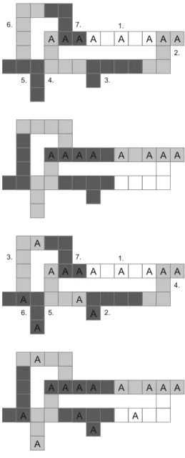
Anyway, Figs.2and3, containing the same gird-like geography with holes (e.g.
lakes), show that employing the crack principle in favor of party Adoes not result in a party Aoptimal districting.6In particular, it can be verified that the geography depicted in Figs.2and3admits just these two feasible districtings from which the crack principle chooses the districting of Fig.2,7while the partyAoptimal districting
5 Obviously, the real-life structure is even more complex, the distribution of partyAandBvoters differ county by county, and there are further restrictions on the set of admissible districts.
6 In the unlabeled squares we have partyBvoters.
7 The numbers close to the districts indicate a possible ordering in which the districts can be chosen based on the crack principle.
Fig. 2 Employing the crack principle
A
A A
A
A A A A
1.
3.
6.
2.
5. 4.
7.
Fig. 3 PartyAoptimal districting
A
A A
A
A A A A
Fig. 4 Employing the pack and crack principle
A A A
A
A
A A
A
A A A A
A
1.
2.
3.
4.
5.
6.
7.
Fig. 5 PartyAoptimal districting
A
A A
A A
A
A A
A
A A A A
A
is shown in Fig.3. Figures2and3improve on the respective example inPuppe and Tasnádi(2009Fig. 2) by pointing out that any implementation of the crack principle results for some problems in a non partisan optimal districting.
We still might hope that by a clever combination of packing and cracking we could obtain a party Aoptimal districting. The pack and crack principle requires that we draw districts sequentially in a way that the number of wasted votes by party A is decreasing; where in case of a cracked district the number of wasted votes by party Aequals the number of partyAvoters not needed for winning the respective cracked district, while in case of a packed district the number of wasted votes by partyAequals
the number of party Avoters in the respective packed district. However, Figs.4and 5show that the pack and crack principle does not always result in a partyAoptimal districting since the geography in Figs.4and5admits just two districtings, the pack and crack principle results in the districting depicted in Fig.4, and Fig.5contains the partyAoptimal districting.
To obtain a heuristic algorithm, the original problem might be simplified in some way. However, to develop a procedure for finding an optimal partisan districting is beyond the scope of this study.
References
Altman M (1997) Is automation the answer? the computational complexity of automated redistricting.
Rutgers Comput Law Technol J 23:81–142
Altman M, McDonald M (2010) The promise and perils of computers in redistricting. Duke J Const L &
Pub Pol’y 5:69–112
Bação F, Lobo V, Painho M (2005) Applying genetic algorithms to zone design. Soft Comput 9:341–348 Bozkaya B, Erkut E, Laporte G (2003) A tabu search heuristic and adaptive memory procedure for political
districting. Eur J Oper Res 144:12–26
Chou C-I, Li SP (2006) Taming the gerrymander-statistical physics approach to political districting problem.
Phys A 369:799–808
Garey MR, Johnson DS (1979) Computers and intractability: a guide to the theory of NP-completeness.
W.H. Freeman and Company, San Francisco
Garfinkel RS, Nemhauser GL (1970) Optimal political districting by implicit enumeration techniques.
Manag Sci 16:495–508
Hess SW, Weaver JB, Siegfeldt HJ, Whelan JN, Zitlau PA (1965) Nonpartisan political redistricting by computer. Oper Res 13:998–1006
Jensen I (2003) Counting polyominoes: a parallel implementation for cluster computing. In: Proceedings of the international conference on computational science, part III. (Lecture notes in computer science), vol 2659. Springer, Melbourne, pp 203–212
Kalcsics J (2015) Districting problems. In: Laporte G, Nickel S, Saldanha da Gama F (eds) Location science.
Springer, Berlin, pp 595–622
Lewenberg Y, Lev O (2016) Divide and conquer: using geographic manipulation to win district- based elections. In: COMSOC-2016, Toulouse. https://www.irit.fr/COMSOC-2016/proceedings/
LewenbergLevCOMSOC2016. Accessed 31 July 2016
Mehrotra A, Johnson EL, Nemhauser GL (1998) An optimization based heuristic for political districting.
Manag Sci 44:1100–1114
Nagel SS (1972) Computers and the law and politics of redistricting. Polity 5:77–93
Puppe C, Tasnádi A (2009) Optimal redistricting under geographical constraints: why ‘pack and crack’
does not work. Econ Lett 105:93–96
Ricca F, Simeone B (2008) Local search algorithms for political districting. Eur J Oper Res 189:1409–1426 Ricca F, Scozzari A, Simeone B (2008) Weighted Vornoi region algorithms for political districting. Math
Comput Model 48:1468–1477
Ricca F, Scozzari A, Simeone B (2011) Political districting: from classical models to recent approaches.
4OR-Q J Oper Res 9:223–254
Tasnádi A (2011) The political districting problem: a survey. Soc Econ 33:543–553 Vickrey W (1961) On the prevention of gerrymandering. Polit Sci Q 76:105–110