Distributed solution of large MILP problems applied to the analysis and control of complex
dynamical systems
J´anos Rudan1, Ton van den Boom2 and Katalin Hangos3
1Faculty of Information Technology, P´azm´any P´eter Catholic University
2Delft Center for Systems and Control, Delft University of Technology
3Computer and Automation Research Institute, Hungarian Academy of Sciences E-mail: rudan.janos@itk.ppke.hu, A.J.J.vandenBoom@tudelft.nl, hangos@sztaki.hu
Abstract—In this paper a set of techniques are presented to solve Mixed Integer Linear Programming (MILP) problems for the model predictive control of complex dynamical systems.
Our aim is to reduce the amount of dealy in railway networks using dynamic traffic management by the rescheduling of trains.
Due to the size of the emerging MILP problem and the given constraints on solution time, a thorough analysis of different MILP solution techniques was necessary. It has been proven that a significant speedup of the solution time can be achieved by the proper restructuring of the matrices of the MILP problem. The simulation results also confirm the effectiveness of the proposed control technique.
Keywords-Mixed Integer Linear Programming; railway scheduling; optimization based control
I. INTRODUCTION
Controlling complex dynamical systems with the help of optimization techniques is a well-known technique. Especially the developments in the field of Model Predictive Control (MPC) gives us the opportunity to exploit the advantages of these approaches. Scheduling problems are emerging when the syn- chronization of the work of several agents is necessary because of the limited capacity of some resources in the system.
In this paper, a model predictive framework is used which gives us the ability to reformulate the dynamic traffic manage- ment of railway networks as a Mixed Integer Linear Program- ming (MILP) problem [1], [2]. The model is formulated in a way that the the order of the trains using the critical resource (namely the tracks) is controlled by binary variables. During the optimization this set of binary variables is determined while minimizing the given cost function.
The proposed technique is capable of predicting a given net- work’s future behavior in case of a cyclic timetable and find an optimal rescheduling of the trains to minimize the summarized delay in the network along the prediction horizon.
II. FORMULATING THE MODEL
Consider a railway network having a periodic timetable with cycle time T. In case of nominal operation the trains follow a pre-scheduled route repeated in everyTminutes where the order of the trains on the tracks is naturally defined by the schedule. If a delay is introduced into the network forcing it to deviate from the
nominal operation, we call the resulting schedule as perturbed mode.
In this section only a short review of the model will be dis- cussed. More detailed explanation of the model (constraints, def- inition of the model predictive control task, MILP-formulation) can be found in [3], [4].
A. Modelling the trains and the tracks
Let’s say trainiis moving on (virtual) tracki, which begins at (virtual) stationi. Let us note that some of the virtual tracks or stations could refer to the same physical track or station meaning that the number of physical tracks in the network usually smaller than the number of virtual tracks.
Letdi(k)be the departure time of trainifrom its departure station in thekth cycle, and let ai(k)be the arrival time of the same train to the other end of the given track. Let rid(k)and rai(k)be the scheduled (nominal) departure and arrival time of the same train, respectively.
B. Building up the constraint set
The departure and arrival times of the trains have to meet with the following constraints:
• Time schedule constraint:a departure may not occur before its scheduled departure time, so we have to satisfy the timetable constraint
di(k)≥rid(k) (1) whererdi(k)is the scheduled departure time for theith train in thekth cycle. For the arrival time a similar constraint can be expressed:
ai(k)≥ria(k) (2)
• Running time constraint: letti(k)be the running time of theith train. The running time constraint then becomes
ai(k)≥di(k−δii) +ti(k) (3) whereδii = 0if the departure time and the arrival time are in the same cycle andδii =µif there isµcycle difference between departure and arrival.
• Dwell time constraint: let pi be the preceding train of traini, which means that trainiandpi are physically the same train. Letspi(k)be the minimum dwell time between
arrival of trainpiand the departure of traini, then we have to satisfy the dwell time constraint
di(k)≥api(k−δipi) +spi(k) (4) where δipi = µ if the (k−µ)th trainpi arriving at the physical station corresponding to virtual stationicontinues as thekth traini.
• Headway constraints: let Fi(k) be the set of trains that move over the same track and in the same direction as train i, and are scheduled before traini. Let j ∈ Fi(k) and let hij denote the minimum headway time between train j and traini. For each trainj ∈ Fi(k)we have headway constraints for both departure and arrival
di(k)≥dj(k−δij) +hij+uij(k)β, ∀j∈ Fi(k) dj(k−δij)≥di(k) +hij+ (1−uij(k))β,∀j∈ Fi(k)
(5) ai(k)≥aj(k−δij) +hij+uij(k)β, ∀j∈ Fi(k) aj(k−δij)≥ai(k) +hij+ (1−uij(k))β,∀j∈ Fi(k)
(6) whereβis a large negative number (soβ 0) anduij(k) is a binary variable. Note that for uij(k) = 0, the con- straints (5.a) and (6.a) will be active, and foruij(k) = 1, the constraints (5.b) and (6.b) will be active.
• Meeting constraints: let Wi(k) be the set of trains that move over the same track and in the opposite direction as traini, and are scheduled before traini. Letj∈ Wi(k)and letwijdenote the minimum separation time between arrival of trainjand departure of traini. For each trainj∈ Wi(k) we have separation constraint
di(k)≥aj(k−δij) +wij+uij(k)β, ∀j∈ Wi(k) dj(k−δij)≥ai(k) +wij+ (1−uij(k))β,∀j∈ Wi(k)
(7) where the role ofβ and uij(k)is similar to the previous case.
It should be noted that during nominal operation allδijvalues are equal to zero or one, but in perturped operation other values are also possible. For sake of simplicity, we will consider only the case whenδij ={0,1}which means thatµmax= 1.
C. Model predictive control and MILP formulation
As it is defined previously, let us consider a network havingn train runs (or shortly trains), and define the following vectors:
z(k) =
di(k)
... dn(k) a1(k)
... an(k)
∈ R2n; r(k) =
r1d(k)
... rdn(k) ra1(k)
... ran(k)
∈R2n
(8) and the elementsui,j(k)withj∈ Fi(k)orj ∈ Wi(k)can be stacked in one vectoru(k)∈Rnu.
The goal of the model predictive controller is to minimize the sum of all delays, and so we come to the object function (or performance index):
J(k) =
Np
X
j=0 n
X
i=1
σi
zi(k+j)−ri(k+j) +
nu
X
l=1
ρlul(k+j)
!
(9) Here Np is the prediction horizon, andσi,ρl are weighting scalars. The first term of (9) is related to the sum of all predicted departure and arrival delays, and the second term denotes the penalty for all train orders changes and broken connections during cyclek+j.
Now define the extended vectors
˜ z(k) =
z(k) z(k+ 1)
.. . z(k+Np)
∈R2nNp; ˜u(k) =
u(k) u(k+ 1)
.. . u(k+Np)
∈RnuNp (10) The object function can be rewritten as:
J(k) =cT z˜
˜ u
(11) where c contains all the values σ and ρ. Also the network constraints (1)-(7) can be written using the vectorsz˜andu˜and we obtain:
Az Au
z˜
˜ u
≤b(k) (12) where matrix Az only consists of entries [Az]ij ∈ { −1,0,1}, matrix Au only consists of entries [Au]ij ∈ { −β ,0, β}andb(k)contains the schedule timesrd(k),ra(k), the running timet(k), the dwell timess(k), the heading times h(k), the separation timesw(k)and the past valuesz(k−j), j = 1, . . . , µmax, whereµmaxis the largest cycle shiftµin the system.
We have now recasted the model predictive control problem into a MILP structure where the objective function is defined in (11) and the constraints in (12).
III. SIMULATION RESULTS
Simulations were done using the model of the Dutch railway system, with a cycle time T = 60min. The network model consists of 41 stations and 118 tracks. In the timetable only the international and interregional trains are included, the local trains are excluded. For the simulationsNp = 2 is selected, so the prediction is done for 2 hours in the future.
The generated problem has 26712 constraints and 5316 vari- ables from which 1728 are continous variable (departure and arrival times) and the remaining 3588 are binary.
A. Scenario generation
In order to simulate the pertubed operation of the system, a new parameter vectorΘp is generated containing all the devi- ations from values in the original schedule described by Θ. It is shown in [5] that the distribution of delays appearing in a train network show a Weibull distribution. In our case delays were generated according to a Weibull-distribution having shape parameter0.8and scale parameter5. Maximal delay was set to 40minand the average introduced delay to10min.
Fig. 1: Comparsion of solution times in case of different MILP problems. CBC outperforms all the other solvers. In the scenarios 8% of trains were selected to be delayed.
A given percentage of the trains were selected from all the trains and the delay values were added to their departure and arrival data, according to two different scenarios:
• case 1: 8% of the trains were selected to be delayed.
• case 2: 20 % of the trains were selected to be delayed.
We usedcase 1in simulations during the selection of the solver (see Section III-B) and we usedcase 2in other tests.
It should be noted that according to available data on average 7.5% of trains are delayed in real life in the Dutch railway network which means that case 2 is related to a much more complex scenario than normal cases.
B. Selecting the proper MILP solver
There are several available MILP solvers both originating from the free software community and commercial ones [6].
Comparsion of the solvers considering the used techniques and algorithms can be found in [7]. Another interesting and con- tinously maintaned review of the solver’s performance can be found at [8].
State-of-art solvers implements stronly heuristic-driven branch-and-cut algorithms to solve MILP problems [9]. Because of their crucial role in the solution speed, heuristics applied in MILP solvers are the subject of extensive research in the recent years [10], [11].
During the present work the following solvers were inves- tigated: from the COIN-OR [12] community: DIP (version 0.83.2), SYMPHONY (version 5.4.4), CBC (version 2.7.6). Also GLPK (version 4.32) and CPLEX (version 12.1) were involved in the tests. The selection process was based on two criteria: on one hand the ability of parallel solution and on the other hand the average solution time.
The solvers were compared based on their average solution time processing a given problem set. The method of the problem generation is detailed in Section III. DIP and GLPK were unable to solve any of the problems in the given time limit. The results of the three remaining solvers can be seen in Figure 1.
Based on the results CBC was selected as the fastest solver.
According to this we used CBC to complete all the other tests and simulations.
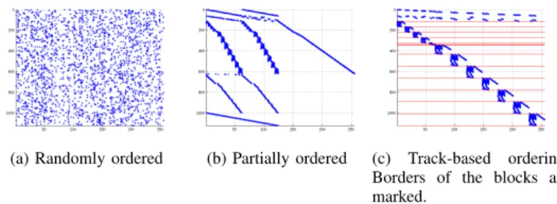
C. Track-based reordering of the constraint matrix
In order to speed up the solution, the constraint matrix has been reordered on a per-track basis.
Reordering on track-basis means that we collect into one block all the constraints and control variables corresponding to a given
(a) Randomly ordered (b) Partially ordered (c) Track-based ordering.
Borders of the blocks are marked.
Fig. 2: Structure of the constraint matrix where the variables are on the x-axis and the equations are on the y-axis. As it can be seen in Fig. 2c. the result of the track-based ordering is a clear block-angular structure.
track. It is clear that the order of the trains on one track is independent of the order on another track. By reordering the constraint set on track-basis we can see similar structure in the MILP formulation. The different constraint blocks correspond- ing to a given track are independent from each other, and the blocks themselves are connected via the continuity contstraints.
In Fig. 2. the reader can see the result of the track-based ordering approach. The formulated blocks can be seen clearly.
Of course any other algorithm generating the constraint set could give some structure to the constraint matrix (as it can be seen on Fig. 2b.) but, among the examined cases the track-based approach gives the best result. The increase in solution speed gained by the proposed reordering is detailed in Secion III-D.
D. Effect of reordering on the solution time
As it was mentioned before, the effect of proper restructuring of the given MILP problem can have huge impact on the solution time. In the present work we selected a track-based ordering which leads to a clear block-angular structure. The following results are verifying that even in the presence of the solver’s preprocessor serious gain can be achieved with proper problem formulation.
In the tests we considered two case. First the columns of the formulated matrices were mixed up randomly. In the other case we built up the same problem’s matrix based but with track-based ordering (see Sec. III-C).
The solution times in both cases for several different scenario can be seen in Fig. 3 for several different scenarios. In the presented case the test set consists of 97 different scenarios. The average solution time was23,97sec(std. dev.14,51sec) without and17,11sec (std. dev.10,13sec) with reordering so the time gain obtained by the reordering was 6.85sec on average (std.
dev.7.04sec) which means a speedup ratio1,407.
E. Results in case of distributed solution
As it is mentioned in Section III-B. several available solvers offers the capabiliy of parallel solution of MILP problems [13].
The simulation result using CBC shows the advantage of the distributed solution. In Fig. 4. the average solution time of a problem set having 100 elements can be seen in case of single- thread and multi-thread setups.
Fig. 3: Solution times in case of a random constraint ma- trix structure or in case of the track-based reordering. The simulation results show that even in the presence of the solver’s preprocessor proper reordering can yield to significant speedup.
Fig. 4: Average elapsed time of solving a MILP with multiple threads on a 4-core (8 cores with Hyper-Threading) computer.
Using 4 threads gives the best result.
During the simulations we used a 4-core computer. The maxi- mal speedup can be achieved if the number of threads is equal to the number of physical cores in the processor.
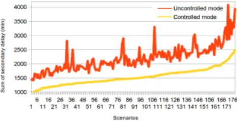
F. Effectiveness of the proposed control technique
To measure the performance of the control technique, the fol- lowing test were completed. Having a given scenario with initial (primary) delays we have simulated the uncontrolled behaviour of the network. During this open-loop simulation all control inputs were set to zero. At the end of the prediction horizon the difference between the result and the reference schedule is calculated as the sum of the delays. For the same scenario we have done the simulation and the calculation of the sum of the delays in controlled mode, too.
The comparsion of the sum of the delays shows the perfor- mance of the control techniques as it can be seen in Fig. 5. We found that the proposed technique can decrease the sum of the delays with 30% compared to the uncontrolled case.
IV. SUMMARY AND FUTURE WORK
In the present paper the details of a previously proposed con- trol technique [4] were investigated. In this framework a general scheduling problem is considered as a MILP problem and solved in an MPC architecture. Due to the computational complexity of the emerging MILP problem and the time constraints on the solution it was necessary to speed up the solution with proper handling of the original problem.
Beyond the selection of a proper solver to solve the MILP problems, the importance of the track-based reordering and the effectiveness of the proposed control technique is shown.
Fig. 5: Effect of optimal reordering of the trains in case of delays. As it can be seen the sum of the delays in the network can be significantly reduced over the control horizon with the help of the proposed control technique.
The general approach - namely the formulation of a schedul- ing problem as a MILP problem in an MPC framework - could be utilized in the optimal control of complex nonlinear systems by using the PWA approximation of the system and the modelling of reaction kinetic networks.
ACKNOWLEDGEMENTS
This work is supported by the Hungarian National Re- search Fund through project K83440 and by the T ´AMOP- 4.2.1.B-11/2/KMR-2011-0002 and T ´AMOP-4.2.2/B-10/1-2010- 0014 grants.
REFERENCES
[1] S. P. Bradley, A. C. Hax, and T. L. Magnanti,Applied Mathematical Programming. Addison-Wesley, 1977.
[2] J. W. Chinneck,Practical Optimization: A Gentle Introduction. Car- leton University, 2009.
[3] T. van den Boom and B. D. Schutter, “On a model predictive control algorithm for dynamic railway network management,” in2nd Interna- tional Seminar on Railway Operations Modelling and Analysis (Rail- Hannover2007), 2007.
[4] T. J. van den Boom, N. Weiss, W. Leune, R. M. Goverde, and B. D.
Schutter, “A permutation-based algorithm to optimally reschedule trains in a railway traffic network,” inIFAC World Congress, 2011.
[5] J. Yuan, “Capturing stochastic variations of train event times and process times with goodness-of-fit tests,” Delft University of Technology, Tech.
Rep., 2007.
[6] A. Lodi and J. T. Linderoth,Encyclopedia for Operations Research and Management Science. Wiley, 2011, ch. MILP Software.
[7] J. T. Linderoth and T. Ralphs, “Noncommercial software for mixed- integer linear programming,” in Integer Programming: Theory and Practice, J. Karlof, Ed. CRC Press, 2005.
[8] Benchmarks for Optimization Software. [Online]. Available:
http://plato.asu.edu/bench.html
[9] M. Galati, “Decomposition methods for integer linear programming,”
Ph.D. dissertation, Lehigh University, 2010.
[10] B. Gendron and T. G. Crainic, “Parallel branch and bound algorithms:
Survey and synthesis,”Operations Research, vol. 42, pp. 1042–1066, 1994.
[11] L. Bertacco, M. Fischetti, and A. Lodi, “A feasibility pump heuristic for general mixed-integer problems,” University of Padova, Italy, Tech.
Rep. Technical Report OR-05-5, 2005.
[12] COmputational INfrastructure for Operations Research. [Online].
Available: http://coin-or.org
[13] T. K. Ralphs,Parallel Combinatorial Optimization. Wiley, 2006, ch.
Parallel Branch and Cut, pp. 53–101.