Numerical simulation of fibre deposition in oral and large bronchial airways in comparison with experiments
Árpád Farkas1,2, Frantisek Lizal2, Jakub Elcner2, Jan Jedelsky2, Miroslav Jicha2
1Centre for Energy Research, Hungarian Academy of Sciences, Konkoly Thege M. 29-33, 1121 Budapest, Hungary
2Faculty of Mechanical Engineering, Brno University of Technology, Technicka 2, Brno 61669, the Czech Republic
Keywords:
man-made vitreous fibres, reconstructed airways, drag force, airway deposition of fibres
Corresponding author:
Árpád Farkas
farkas@fme.vutbr.cz
1 Abstract
Inhaled asbestos fibres have been implicated in causal relationships with increased frequencies of non-malignant pleural disease, asbestosis, mesothelioma and lung cancer.
Replacement fibres are considered to be less harmful, however, their health effects are not fully understood. The objective of the present work was to implement and apply numerical fibre tracking techniques in order to simulate the deposition of fibres in a complex oro-pharyngeal- laryngeal-bronchial system at different inhalation flow rates and compare the results with the outcomes of recent measurements performed in the same geometry. Two different approaches for the estimation of drag force were considered. Simulated deposition efficiency values agreed reasonably well with the experimentally determined values, however, the drag model which considers the anisotropic nature of the geometry of fibres performed better than the one which accounted only for the their non-spherical shape. The highest values of deposition density correlated well with the location of primary lesions observed in pathological studies.
2 1. Introduction
The airways are not only a gas conducting and exchange system but also a route of the entrance of particulate matter into the human body. Inhalation of detrimental aerosols, such as toxic particles, radio-aerosols or some of the bio-aerosols may cause adverse health effects, especially if the inhaled dose is sufficiently high to surpass the capability of different defence mechanisms to eliminate them. On the other hand, medical aerosols play a key role in the management of respiratory diseases like asthma or COPD (chronic obstructive pulmonary disease). However, the desired therapeutic effect can be obtained only if the right amount of medication is delivered to the right place within the airways. Therefore, the biological effects of both the inhaled detrimental and therapeutic aerosols depend on the amount of particles depositing within the airways and spatial distribution of the deposition.
In practice, safe levels of exposure are provided for different proven harmful substances in terms of their concentration in the air. However, not all the inhaled detrimental particles deposit in the airways. Since the biological response depends on the deposited particles, it is of high importance to find the relationship between the particle concentration in the air and the amount of substance deposited within the airways. In addition, health consequences may depend not only on the total amount of deposited substance but also on the spatial distribution of the deposition within different segments of the airways. It has been demonstrated that even low ambient particle concentrations can lead to high local doses in specific sites of the airways (Balásházy et al, 2003). Therefore, it is indicated to quantify the deposition not only in the whole respiratory system but also in its distinct segments.
A significant effort has been spent in the last decades to quantify the fraction of inhaled particles depositing within the human airways. The development of different measurement methods allowed us to perform in vitro (and to a smaller extent also in vivo) experiments of particle transport and deposition within the airways. By the same token, the continuing increase of computing capacities and the more and more sophisticated algorithms and software promoted the rapid increase of the number of simulation works focusing on the quantification of airway deposition of the inhaled aerosols. Most of the related experimental and numerical works aimed to characterize the deposition of spherical particles. In contrast, much less knowledge on the airway deposition of non-spherical particles has accumulated so far. One of the reasons is the more complicated aerodynamic behaviour of non-spherical particles compared to the spherical ones.
Fibre shaped particles are a distinct category of inhaled non-spherical aerosols. Asbestos fibres, especially amphibole asbestos types such as crocidolite, tremolite and amosite were
3
recognised to cause mesothelioma, lung cancer, asbestosis and non-malignant pleural disease (Barbieri et al, 2012; Bernstein et al, 2013). Therefore, their mining gradually ended in most of their major mining sites (South Africa, Australia and Bolivia). Among the replacement fibres, man-made inorganic vitreous fibres are considered to be less biopersistent and less harmful, but the consequences (especially the long term ones) of the inhalation of such fibres are far from being fully explored and understood. Based on the current knowledge the International Agency for Research on Cancer declared slag wool, rock and glass fibres as non- carcinogenic and ceramic fibres as potentially carcinogenic (IARC 2002). In the European Union the occupational exposure limit for man-made vitreous fibres is 1 fibre/ml (SCOEL 2012). As mentioned before, the missing bridge between the macroscopic exposure expressed in terms of particle concentration and the related health effects can be the quantification of the fraction of fibres depositing within the airways.
There is only a limited number of experimental works in the open literature focusing on the deposition of fibres within the human airway system. In vivo deposition experiments have both technical and ethical barriers. In vitro deposition experiments have been performed with various fibre types and different airway replicas by Myojo (1990), Sussman et al (1991), Myojo and Takaja (2001), Su and Cheng (2005), Zhou et al (2007), Su and Cheng (2009) and Belka et al (2018), among others.
The number of computational works focusing on the airway deposition of the inhaled fibres is significantly higher and the complexity of the approaches spans a large spectrum. Capturing of complex flow features in the complicated geometry of the airways and describing both translational and rotational motion of fibres as a result of acting forces which have more complicated forms compared to the case of spherical particles is mathematically challenging and computationally demanding. Therefore, earlier works assumed idealized geometries of the airways and simplified cases of fibre motion. Jeffery (1922) was probably the first to theoretically address the motion of fibres by describing the behaviour of ellipsoids immersed in viscous fluids. Harris and Freaser (1976) have developed an analytical airway deposition model of fibres in both laminar and turbulent flows. Cai and Yu (1988) deduced mathematical relationships for inertial and interceptional deposition of fibres in idealized single bifurcation.
The same deposition mechanisms were considered in a single idealized bifurcation by Zhang et al (1996). For this purpose the authors applied CFD techniques. Balásházy et al (2005) used a combination of stochastic analytical and CFD models to characterize the regional deposition of fibres in the whole airways and local patterns of fibre deposition in a single symmetric
4
bifurcation. They have used sedimentational and impactional equivalent spherical diameters for parallel, perpendicular and random orientation of fibres.
Later, the increase of computer capacities allowed the numerical modelling of fibre transport and deposition in larger segments of airways and implementation of more complex fibre tracking algorithms. For instance, a multigenerational model of the tracheobronchial tree built by sequentially bifurcating tubes was used by Tian and Ahmadi (2013) to perform CFD computations of slender fibre deposition. A computational model for the coupled translational and rotational motions was implemented to analyse the effect of fibre size, airflow and airway morphology on the deposition of fibres.
By the enhancement of the resolution of medical imaging techniques (MRI – magnetic resonance imaging, CT – computed tomography) it became possible to reconstruct larger and larger parts of the upper and central airways and to study the deposition of fibres in more realistic airway geometries including the oral and nasal cavities. A complex oro-pharyngeal- laryngeal-tracheobronchial geometry down to lobar bronchi was used by Feng and Kleinstreuer (2013) to simulate the deposition of ellipsoidal particles by applying mathematical equations for drag, lift and Brownian forces. Deposition of fibres in the human nasal airways reconstructed from medical images was analysed by Inthawong et al. (2008), Wang et al (2008), Inthawong et al (2013), Dastan et al (2014), Shanley et al (2018), among others.
In most of the numerical studies the outcomes of numerical simulations were not compared to the results of experimental measurements or the measurement results were not obtained in the same airway geometry. The works of Inthawong et al (2008) and Feng and Kleinstreuer (2013) are among the few exceptions. The objective of the present work is to implement numerical models of fibre tracking and apply them to quantify fibre deposition in exactly the same reconstructed oropharyngeal-laryngeal-tracheobronchial airway geometry and the same fibre properties and inhalation conditions which were applied in the recent work of Belka et al (2018). In addition, the present work aims to compare the numerical results also to other experimentally measured fibre deposition data available in the open literature.
5 2. Methods
2.1 Basic approach and assumptions
In the present work, a CFPD (computational fluid and particle dynamics) method has been applied to model the transport of the inhaled air and fibres within the airways and to quantify the deposition of fibres. An Euler – Lagrange approach has been implemented which implied the tracking of individual fibres in the computed airflow field treated as a continuum. One way coupling between the fibres and air was assumed, that is, the airflow influenced the fate of fibres, but the fibres had no effect on the airstreams. Since the computations were performed in an existing geometry, the main steps of the numerical simulations included the creation of a numerical mesh, computation of airflow field and computation of fibre trajectories and deposition. From now on, we provide a description of the geometry and the main steps of the modelling.
2.2 Model airway geometry
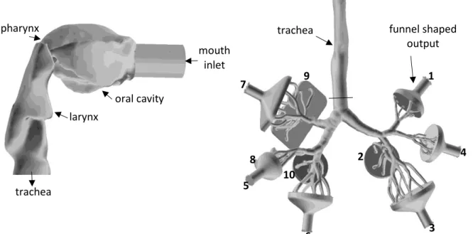
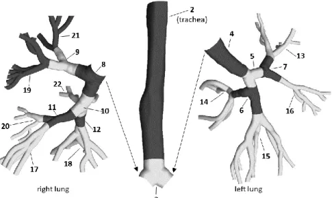
In this work the transport and deposition of fibres was numerically simulated in a model airway geometry including the oral cavity, pharynx, larynx, trachea and bronchial airways down to the 7th bronchial generation (if the numbering begins with the trachea as generation 0). The tracheobronchial part of the geometry is based on the reference model of Schmidt et al (2004), while the upper airway part was acquired from the Lovelace Respiratory Research Institute (Albuquerque, MM, USA, Cheng et al (1997). A detailed description of the airway geometry can be found in Lizal et al (2012). The rationale for choosing this digitized geometry for the current numerical simulations of fibre deposition is that its physical counterpart has been used in the past to quantify the deposition of spherical aerosols (Lizal et al, 2015), and recently to experimentally measure the deposition of glass fibres at different inhalation flow rates (Belka et al. 2018), thus a direct comparison of experimental and numerical deposition results is possible. Figure 1 demonstrates separately the geometry of the upper airways (left, side view) and the multigenerational tracheobronchial tree (right, anterior view) used in this study. To comply with the experimental setup used in Belka et al (2018) a circular pipe with diameter of 2 cm was attached to the mouth inlet and 10 output segments with ‘funnel-like’ shapes were added.
6
Figure 1. Side view of the oropharyngeal-laryngeal (left) and anterior view of the tracheobronchial (right) parts of the model airway geometry. For the sake of visibility the upper airways were removed from the rest of the geometry, enlarged (3×) and rotated (90° counter clockwise around the gravity axis). For a better identification the outlets are numbered from 1 to 10
2.3 Computational mesh
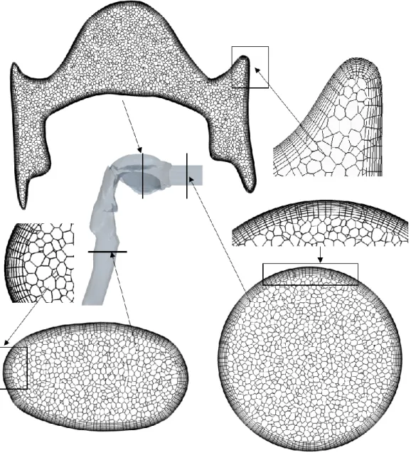
The airway geometry has been divided into discrete computational cells by the help of Star- CCM+ commercial software. Hybrid meshes containing polyhedral cells in the core region of the domain and prismatic cells near the wall boundary were considered. The density of the near-wall mesh was non-uniform, the size of the cells decreasing in the direction of the wall to accurately describe the airflow and fibre behaviour in the near-wall region. The first mesh point near the wall was set to satisfy the y+<1 condition (y+ – non-dimensional wall distance). The wall spacing fulfilling this condition was estimated before the construction of the meshes (White 2003) and verified after the completion of the flow computations. Two dimensional cross sections of the mesh are depicted in Figure 2 highlighting special features of the mathematical grid at different locations of the airway geometry.
mouth inlet oral cavity
pharynx
larynx
trachea
trachea funnel shaped
output 1
2 4
3 5
6 7
8
9
10
7
Figure 2. Cross sections of the applied computational mesh at different locations of the airway geometry
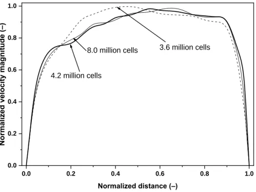
Significant effort has been spent to ensure grid independency of the results. The grid independency test was performed by gradually increasing the mesh size, while monitoring the velocity magnitude and turbulent kinetic energy contours downstream of the laryngeal zone where complex flow phenomena occur (e.g. recirculating regions, free-shear layers, mean streamline curvature, Koullapis et al. 2018). Even the coarsest mesh satisfied the above condition for y+. The tests were completed for 15 and 50 L/min inlet flow rates. The outcome of the test was that the mesh containing about 4.2 million computational cells accurately describes the flow and it is computationally less expensive than the finest mesh, thus this mesh was kept for the rest of the flow field computations and for the particle trajectory simulations.
8
Figure 3 depicts a sample test result for the velocity profiles along a diameter of tracheal cross section marked in Figure 1 (right panel) for meshes containing 3.6, 4.2 and 8.0 million cells.
Figure 3. Normalized velocity magnitude profiles along a tracheal cross-sectional diameter for three different numerical mesh sizes
2.4 Flow field computations 2.4.1 Physical model
The inhaled airflow was modelled in the oropharyngeal-laryngeal-bronchial geometry shown in Figure 1. In line with the experimental conditions in Belka et al (2018), in this work steady inspiratory flows with 15, 30 and 50 L/min mouth inlet flow rates were assumed. The density of the air was 1.23 kg/m3, while its viscosity was 1.79×10⁻⁵ kg/(m s). Based on our earlier works (Farkas et al. 2006, Farkas et al. 2018) and also the recent benchmark work (the SimInhale benchmark case, Koullapis et al. 2018) in the airway geometry identical to the present one the carefully validated RANS k-ω turbulence models with appropriate mesh and settings can be suitable for the modelling of the airflow in this region of the airways. In this work the k-ω SST model with the default model constants, but with low-Re correction for the estimation of turbulent viscosity was used.
2.4.2 Boundary conditions
The boundaries of the model consisted of an inlet, ten outlets and a wall surface (see Figure 1).
In conformity with the experiments described in Belka et al (2018) uniform air velocity profiles
0.0 0.2 0.4 0.6 0.8 1.0
0.0 0.2 0.4 0.6 0.8 1.0
3.6 million cells 8.0 million cells
4.2 million cells
Normalized velocity magnitude (–)
Normalized distance (–)
9
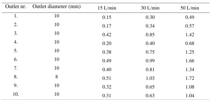
were prescribed at the ten circular outlets. The values of the outlet velocities together with outlet diameters are provided in Table 1 for 15 L/min, 30 L/min and 50 L/min inhalation flow rates at the mouth inlet. The numbering of the outlets is identical to the one demonstrated in Figure 1. It is worth noting that the diameters in Table 1 are not the diameters of the individual bronchi, but the diameters of the cylindrical parts of the funnel shaped outlets. Also note that the velocity values in Table 1 are absolute values and all outlet velocity vectors pointed outside the geometry, thus velocity values in Table 1 were considered with negative sign.
Table 1. Outlet diameters and air velocities at the ten outlets of the airway geometry in Figure 1 for 15, 30 and 50 L/min inhalation flow rates
Outlet air velocity (m/s)
Outlet nr. Outlet diameter (mm) 15 L/min 30 L/min 50 L/min
1. 10 0.15 0.30 0.49
2. 10 0.17 0.34 0.57
3. 10 0.42 0.85 1.42
4. 10 0.20 0.40 0.68
5. 10 0.38 0.75 1.25
6. 10 0.49 0.99 1.66
7. 10 0.40 0.81 1.34
8. 8 0.51 1.03 1.72
9. 10 0.32 0.65 1.08
10. 10 0.31 0.63 1.04
Zero gauge pressure was prescribed at the mouth inlet and the operating pressure was the normal atmospheric pressure. The value of turbulent intensity was set to 1% at the outlets and to 6, 5 and 4% at the mouth inlet, corresponding to 15, 30 and 50 L/min inlet flow rates, respectively. The hydraulic diameter was 2 cm at the mouth inlet and took values similar to the corresponding cylindrical tube diameters at the outlets (provided in Table 1). In addition, no- slip condition (zero air velocity) was assumed at the wall boundary.
2.4.3 Numerical model
Transport equations of mass, momentum, turbulent kinetic energy and its dissipation rate were solved numerically by the solver of the commercially available FLUENT CFD code (version 19.1, part of ANSYS 19.1 software). A finite volume method has been applied to numerically solve the mathematical equations describing the air flow. Each algebraic equation was
10
discretized and written for every control volume. The resulting set of equations were linearized and solved using a Gauss – Seidel iteration method in conjunction with an algebraic multigrid (AMG) technique for the acceleration of the solution. In the present work the pressure based solver (momentum and pressure are the primary variables) with segregated algorithm (pressure correction and momentum equations are solved sequentially) was applied. All the field variables were interpolated to the faces of the control volumes by using second order upwind schemes. Gradients of solution variables at cell centres were determined by the least-squares cell-based approach which is the recommended scheme for polyhedral cells to avoid false diffusion. Gradients of solution variables at cell faces were computed using multidimensional Taylor series expansion. The PRESTO! (Pressure Staggering Option) algorithm was applied to find out cell-face pressures. This algorithm staggers the mesh so that pressure and velocity variables are not co-located. In this way cell-face pressure is directly computed instead of interpolating it from cell centre values, avoiding interpolation errors and gradient assumptions (e.g. zero normal pressure gradient at wall). This method provides accurate results for strongly curved domains, such as parts of the oral cavity and larynx. The pressure-velocity coupling numerical algorithm for the derivation of pressure correction equation was the SIMPLE (Semi- Implicit Method for Pressure-Linked Equations) algorithm, which is a robust numerical scheme for steady flows.
2.4.4 Solution monitoring and controlling
At every iteration step, scaled residuals were computed and monitored for each conserved variable. In some cases convergence was sped up by fine tuning the under-relaxation factors.
About 50,000 iteration steps were needed. Values of all scaled residuals fell at least three orders of magnitude during the flow simulations, had final values below 10–4 and remained nearly constant over the last 5000 iteration steps. In addition to monitoring residual histories, overall mass balance was also verified to ensure a net imbalance less than 1% of the smallest flux through the domain boundary. All the computations were performed on 15 cores of Intel Xeon E5-2690 processors of the computing cluster of Brno University of Technology.
2.5 Modelling of fibre motion
Setting up the appropriate physical and suitable numerical models accounting for the particularities of the airways and for the special characteristics of the fibres are indispensable conditions of obtaining reliable airway deposition results. In the followings the main properties
11
of the studied fibres, and the physical, mathematical and numerical models of fibre trajectory computations are presented in separate subsections.
2.5.1 Fibre properties
In order to ensure that numerical results can be directly compared with experimental measurements, the physical properties of fibres were adopted from the work of Belka et al (2018). The density of fibres was 2560 kg/m3, which corresponds to the density of glass fibres in the above work. The diameter of the modelled fibres was 1.03 m and three lengths were considered for each flow rate. The values of fibre length and standard deviation were 17±3.6 m, 17±3.2 m and 20.9±4.5 m at 15 L/min, 21.7±6.3 m, 21.2±6.5 m and 19.2±5.1 m at 30 L/min and 22.1±5.9 m, 23.2±6.7 m and 27±9.2 m at 50 L/min inhalation flow rate. Similar to the experimental measurements, separate deposition simulations were performed for every fibre size distribution and the three deposition results for the same flow rate were averaged.
2.5.2 Physical and mathematical model of fibre dynamics
As mentioned before, a Lagrangian method was applied to track the particles within the airways. This implies that the particle force balance equation is written and solved for every individual particle. To reliably estimate the fate of fibres after the inhalation it is essential to accurately describe the forces acting on them while being transported by the inhaled airstreams within the airways. In its most general form the force balance equation can be written as
( ) (1 )
p
D p o
p
du F u u g f
dt
, (1)
where u and up denote the velocity of the air at the location of the particle and the velocity of the particle, respectively. By the same token isthe density of air and p the density of the particle and fo represents all the other forces acting on the unit mass of particle (e.g. Brownian force). The term FD(u-up) symbolizes the drag force of unit mass with
2
18 Re 24
ps
D D
p ps
F C
d
. (2)
In equation (2) dps is the volume equivalent spherical diameter of the particle, that is, the diameter of a sphere having the same volume as the volume of the fibre. In addition, CD
represents the drag coefficient, while denotes the dynamic viscosity of the air. The determination of the drag coefficient for fibres is not a trivial task being extensively studied in the open literature. As a result, a large number of empirical formulas for CD have been derived.
12
The principles behind the selection of the drag models used in this study were their proven capability to accurately describe the motion of fibres in the Reynolds regimes which dominate fibre transport within the airways and the possibility to implement them into the FLUENT 19.1 solver (ANSYS 19.1) in form of user defined functions (UDFs).
For non-spherical particles the drag coefficient is usually expressed either as a function of particle Reynolds number or as a function of Reynolds number and one or more shape factors.
Shape factors are dimensionless numbers introduced in the expression of drag force to account for the non-spherical shape. There are several types of shape factors used in the literature. One of them is sphericity () introduced by Wadell (1933). Sphericity is defined as a ratio of the surface area of the volume-equivalent-sphere (sphere with the same volume as the volume of the particle) to the actual surface area of the particle (A)
2
dps
A
. (3)
Mathematical equations of the drag coefficient valid for different ranges of Reynolds number (Re) and have been provided by several authors, e.g. Ganser (1993), Haider and Levenspiel (1989) and Hartmann et al (1994), among others. The formalism presented by Haider and Levenspiel (1989) was incorporated into the FLUENT solver and it will be used also in this paper. Based on this approach the drag coefficient (CD) can be expressed as
2 3
1
4
24 Re
(1 Re )
Re Re
t ps
D ps
ps ps
C t t
t
, (4)
where
2 1 exp(2.3288 6.4581 2.4486 )
t ,
2 0.0964 0.5565
t ,
2 3
3 exp(4.905 13.8944 18.4222 10.2599 )
t and
2 3
4 exp(1.4681 12.2584 20.7322 15.8855 )
t . (5)
In equation (5) Reps denotes the Reynolds number associated with the particle yielded by Reps pdps u up
, (6)
where is the dynamic viscosity of the air.
According to Haider and Levenspiel (1989) their empirical equations perform well for isometric particles with shape factors higher than 0.67, but fit poorer for shape factors lower than 0.23. It is worth noting that for the present fibres with dimensions presented in subsection
13
2.5.1 takes values between 0.43 and 0.5. Inthawong et al (2008) have demonstrated that equation 4 yields reasonable results for cylindrical fibres with aspect ratios (length/diameter) up to around 15-20. The aspect ratio of our fibres varied between 16.5 and 26.2, thus the above approach may provide fairly good results, but a model accounting for non-isometric nature of fibres is physically sounder and most probably also more accurate. Therefore, in addition to the Haider and Levespiel model (‘H-L model’) we have adopted the empirical model of Tran - Cong et al (2004) and hereon we will call it the ‘T-C model’. In the T-C model particle circularity (c) and the ratio of surface-equivalent diameter to the volume-equivalent diameter (r=dA/dps) are taken into account to assess the drag coefficient. Circularity replaces and it is defined as
A p
c d P
, (7)
where dA is the diameter of the surface-equivalent sphere, that is, a sphere with the same surface area as the non-spherical particle. In equation (7) Pp denotes the projected perimeter of the particle in its direction of motion. By this notations the expression of drag coefficients can be written as
2 0.687
1.16
24 0.15 0.42
1 ( Re )
Re 1 42500( Re )
D ps
ps ps
C r r r
c c r
. (8)
As the orientation of the fibre and particle Reynolds number may change, the value of CD given by equation (8) must be recalculated at every time step of the particle tracking.
2.5.3 Implementation of numerical particle tracking model
Tracking of individual fibres was performed by the integration of the equation of motion (equation 1). Due to the large sizes of our fibres Brownian motion was neglected. Electric forces were also not considered. This assumption matches the conditions in the experiments of Belka et al (2018), where a charge neutralizer was used to obtain electrically neutral fibres.
Since the H-L formalism is included in FLUENT DPM (discrete phase model), the implementation of equations (3) – (6) was performed by simply choosing the non-spherical drag law and providing the input value of the shape factor (). The T-C model (eq. 7 – 8 in conjunction with equation (9) were implemented by the help of a user defined function written in C++ programming language attached to FLUENT solver. As mentioned before, the orientation of fibre is needed at every time step of particle tracking. Since the current model does not include the computation of torque, the orientation is not calculated. Instead, a random
14
orientation was assumed, which is a reasonable first approach in the complex turbulent flows in the upper and large bronchial airways. In reality, the orientation of fibres is a multiparametric function, which can be deduced by systematic experiments performed in airway geometries with various degrees of complexity starting from simple straight tube and continuing with single bifurcations and more and more complex airway geometries. Similarly, the experiments should start with simple channel flow, laminar flows, then transitional and fully complex turbulent flows. Such efforts are in progress within the research group of the authors. For the selection of the orientation at every time step a random number generator has been used.
Turbulent dispersion may play an important role in fibre deposition, thus the discrete random walk model of FLUENT has been enabled during the particle trajectory simulations. The numerical integration of particle force balance equation was performed by an automated scheme, which switches in an automated fashion between numerically stable lower order schemes and higher order schemes, which are stable only in a limited range. As a higher order scheme the Runge – Kutta method was used, while an implicit tracking method was used as a lower order scheme. The maximum relative error of the tracking procedure was set to10–5. The time step of the numerical integration was lower than the Stokes and turbulent time scales.
Further reduction of time step did not cause significant change in the deposition results. The fibres were released at the geometry inlet (mouth inlet, see Figure 1). Tracking of 100,000 individual fibres was necessary during each run to ensure statistically accurate deposition results. Switching to 1,000,000 particles would modify the deposition fraction values by less than 1% relative to the values obtained for 100,000 fibres.
2.5.4 Quantification of fibre deposition in different airway segments
In this work, the deposition of particles was quantified in terms of deposition fraction and deposition efficiency. Deposition fraction is the ratio of the number of particles deposited in a segment to the number of particles entering the whole domain. Deposition efficiency is the ratio of the number of particles deposited in a certain segment to the number of particles entering the same segment. The division of the current airway geometry into distinct segments can be seen in Figure 4. The upper airway part shown in the left panel of Figure 1 is segment 1.
15
Figure 4. Segmentation and numbering of the modelled airways. The geometry has been cut at the left and right main bronchi for a better visualisation
In most of the cases, in the open literature the deposition fraction in the upper airways and large bronchi is usually expressed as a function of impaction parameter or Stokes number. The impaction parameter is defined as
2
IPdae Q, (9)
where Q denotes the inhalation flow rate and dae is the equivalent aerodynamic diameter. Stokes number is
2
18
pd Uae
Stk D
, (10)
where, as in equation (2), p and are the density of particle and the viscosity of air, respectively. By the same token, U denotes the mean velocity and D defines the equivalent mean diameter of the given airway. In the upper airways (segment 1) the mean velocity is computed from
2
U 4Q
D
(11)
and the mean diameter is 2(V )1/2
D L , (12)
16
where V is the volume of the upper airways and L is the length of the centreline path.
In the individual branches (segments 2 and 4) and single bifurcations (segments 3 and 5 – 12) of the tracheobronchial tree U represents the mean velocity in the single branch or in the parent branch, respectively. By the same token, D is the mean diameter of the same single branch or parent branch. In the segments containing multiple airway generations (segments 13 – 22) the mean diameter was computed by first calculating the output equivalent diameter (mean of output diameters), then averaging the input diameter with the output equivalent diameter. The mean velocity in such segments was calculated based on the flow rate in that segment and the above described mean diameter.
The equivalent aerodynamic diameter of fibres in equations (9) and (10) can be calculated based on formulas provided by different investigators (e.g. Stöber, 1972;
Harris and Fraser, 1976; Prodi et al, 1982; Gonda and Abd El Khalik, 1985). In this study, the formalism of Stöber (1972) has been used by computing the equivalent diameter as
0 p
ae ps
d d
, (13)
where dps is the volume-equivalent sphere diameter, 0 is the density of water and is the dynamic shape factor. This factor depends on the shape and size of the particle but also on its orientation. The parallel orientation of a fibre with the direction of the flow yields the highest value for dae, while perpendicular orientation provides the lowest equivalent diameter. For random orientation, the dynamic shape factor can be expressed as a combination of its parallel ( ) and perpendicular () components (Fuchs, 1964)
1 1 2
3 (14).
The two components of the dynamic shape factor can be computed assuming that the fibre behaves as a prolate spheroid (Baron and Willeke, 2001). The corresponding formulas are
2 1/3
2 2 1/ 2 2 1/ 2
(4 / 3)( 1)
((2 1) / ( 1) ) ln( ( 1) )
(15)
and
2 1/3
2 2 1/ 2 2 1/ 2
(8 / 3)( 1)
((2 3) / ( 1) ) ln( ( 1) )
, (16)
where is the fibre’s aspect ratio.
17 3. Results and discussion
Based on our simulation results the mouth-throat deposition fraction values yielded by the T-C model were 1.1, 2.1 and 4.2% at 15, 30 and 50 L/min inhalation flow rates, respectively.
The same deposition values yielded by the H-L model were 1.6, 3.6% and 8.3%. By the same token, the application of T-C drag model led to tracheobronchial deposition fraction values of 3.8% (at 15 L/min), 6.3% (at 30 L/min) and 8.4% (at 50 L/min), while the use of the H-L model resulted in 10.6% (at 15 L/min), 20.3% (at 30 L/min) and 33.7% (at 50 L/min) tracheobronchial deposition fraction values. As the above results demonstrate, regional deposition values obtained by the T-C model were consistently lower than those yielded by the H-L model.
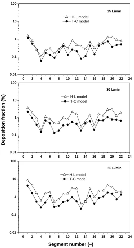
Figure 5 depicts the deposition fraction values computed by the two numerical models in the distinct segments of the airways (presented in Figure 4) at 15, 30 and 50 L/min inhalation flow rates. As expected, the deposition fractions increased with the increase of inhalation flow rate due to the more intense deposition of fibres by inertial impaction. The figure demonstrates that the curves have quite similar shapes, but the values obtained by the H-L model are systematically higher than those corresponding to the T-C model. This is due to the higher values of the drag force in case of the T-C model. The H-L model, which completely disregards the orientation of the fibres, is a deterministic model. On the contrary, the values of the drag force in the T-C model are selected stochastically. Therefore, there is no threshold value of Reps under which the T-C drag force is higher than the H-L drag force, but a post-simulation analysis demonstrated that under the present conditions the T-C model indeed yielded higher drag forces. Concerning the distribution of the deposition among the different airway segments, the highest values of deposition fraction were obtained in the oral airways and in the trachea, but local deposition maxima could be observed also in segments 5 (6 for 50 L/min), 11, 15 and 19. A significant fraction of the fibres that deposited in the oral airways could be found around the throat (pharynx) highlighting the significance of inertial impaction as a dominating deposition mechanism. In the trachea a significant fraction of the deposition was caused by the laryngeal jet (Elcner et al, 2016) enhancing turbulence levels downstream of the larynx and accelerating the fibres. The above mentioned airway segments characterized by higher deposition fractions are the passages towards the outlets 3, 6, 7, 8 (Figure 1), where air velocity is the highest (Table 1). In these regions, higher velocity promoted the deposition of fibres by impaction. In addition, higher air velocity means higher volume of air in unit time (higher flow rate), thus more fibres flowing towards that outlets, which also results in more deposited fibres.
18
At the same time, local deposition minima occurred at segments 4, 7, 13 – 14 and 16. The lower deposition in segment 4 can be explained by the fact that this segment is a single tube and fibres predominantly deposited at bifurcation regions (carinal ridges). Airway segments 7, 13, 14 and 16 are all in the left upper lobe leading to the outlets 1 and 4 (Figure 1), where the air velocity was the lowest (Table 1).
Figure 5. Deposition fractions in airway segments 1 – 22 at 15 L/min (upper panel), 30 L/min (middle panel) and 50 L/min (bottom panel) inhalation flow rates corresponding to the two drag models
Segment number (–)
Deposition fraction (%)
0 2 4 6 8 10 12 14 16 18 20 22 24
0.01 0.1 1 10 100
15 L/min H-L model
T-C model
Deposition fraction (%)
Segment number (-)
0 2 4 6 8 10 12 14 16 18 20 22 24
0.01 0.1 1 10 100
30 L/min H-L model
T-C model
Deposition fraction (%)
Segment number (-)
0 2 4 6 8 10 12 14 16 18 20 22 24
0.01 0.1 1 10 100
50 L/min
Deposition fraction (%)
Segment number (-) H-L model T-C model
19
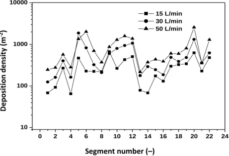
Fibres deposited in the airways interact with the lungs causing continuous generation of reactive oxygen species (ROS) that are related directly to fibre toxicity and effects on DNA and proteins (Shukla et al, 2003). From the perspective of the biological outcome not only the number of human cells affected, but also their spatial distribution is essential. Closely distributed primary damages may be more dangerous than the same number of affected areas distributed sparsely. Therefore, besides the quantification of the deposition distribution of the inhaled fibres in distinct segments of the human tracheobronchial tree, it is plausible to quantify also the deposition density of the inhaled fibres. This can be realized by dividing the computed deposition fractions by the surface area of the airway segment. Figure 6 depicts the computed deposition densities along the 22 airway studied segments. Only the results of the computations using the T-C model are plotted.
Figure 6. Deposition density in airway segments 1-22 at 15, 30 and 50 L/min inhalation flow rates computed by the T-C model
As Figure 6 demonstrates, the distribution of deposition density among the different airway segments is different from the distribution of deposition fraction shown in Figure 5. One of the most important changes can be observed in the first airway segments. The highest deposition fraction characterizing the first segment resulted in one of the lowest deposition densities due to the large surface of the oral cavity and pharynx. The same tendency can be seen in the case of the trachea (segment 2). This might be one of the explanations for the histological finding that carcinoma of the tracheal epithelium is less frequent. On the contrary, a local maximum of the deposition density can be seen at segment 3, which is the region where the trachea branches
Segment number (–)
0 2 4 6 8 10 12 14 16 18 20 22 24
10 100 1000 10000
Deposition fraction (%)
Segment number (-) 15 L/min 30 L/min 50 L/min
Deposition density (m-2 )
20
into the two main bronchi. This bifurcation region coincides with one of the preferential locations of the malignancies caused by particulate matter inhalation reported in histo- pathological studies (e.g. Veeze 1968). Other maxima of the deposition density appear around airway segments 5-6, 11-12 and in segment 20. Two of them are located in the right lung and only one in the left lung. This is also in line with the finding that bronchial carcinomas are more frequent in the right lobes (Garland 1961).
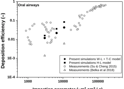
In addition to the analysis of the results of numerical simulations obtained by different drag models and the explanations for the observed trends, it is also useful to compare the numerical results to the results of fibre deposition experiments. This was also one of the aims of the current work. Figure 7 presents simulated and measured values of oral deposition fraction as a function of impaction parameter defined in the Methods section.
Figure 7. Simulated deposition efficiency of fibres (filled symbols) as a function of impaction parameter in the oropharyngeal-laryngeal airways in comparison with experimentally measured values (empty symbols)
Current results were compared to the results of Su and Cheng (2015), who experimentally measured the deposition of glass, TiO2 and carbon fibres and Belka et al (2018), who measured the deposition fraction of glass fibres. Figure 7 demonstrates that in general the deposition fraction values calculated with both drag models are in line with the measured values, especially with the values of Su and Cheng (2015). Compared to the results of Belka et al (2018) the simulated deposition fraction values are higher. Indeed, it was mentioned in Belka et al (2018) that their oral cavity deposition should be considered as a lower bound estimate, because some fibres could remain hidden due to obscuring of small portions of filters by the debris released from the replica wall. In addition, in this region of the airways our numerical
Impaction parameter (m2 cm3 / s)
Deposition efficiency (–)
1000 10000 100000
1E-4 1E-3 0.01 0.1 1
Oral airways
Deposition efficiency (-)
Impaction parameter (m2×cm3/s)
Present simulations W-L + T-C model Present simulations H-L model Measurements (Su & Cheng 2015) Measurements (Belka et al 2018)
21
turbulent dispersion model may overestimate the deposition to some extent. The discrete random walk (DRW) algorithm included in FLUENT does not account for the anisotropic nature of turbulence in boundary layers introducing an over-prediction for the wall normal component of velocity fluctuation (Debhi, 2011). It is also worth noting that in reality the turbulent dispersion of fibres is different from that of spherical particles, however, to the best of our knowledge there is no such numerical model developed for fibres in the open literature.
Simulated tracheal deposition efficiencies as a function of Stokes number are presented in Figure 8 (left panel) in comparison with experimentally measured values of Su and Cheng (2009) and Belka et al (2018). The increase of deposition fraction with the increased Stokes number indicates that deposition by impaction is important also in this region. Again, the numerical results (at least those obtained by the T-C model) are in line with the measurements of Su and Cheng (2009), but they are somewhat higher than the data of Belka et al (2018).
Although turbulent intensity decreases towards the lower end of the trachea (towards the main bronchi) deposition in its upper part is influenced by the higher turbulent levels caused by the laryngeal jet mentioned above. It is likely that the currently used turbulent dispersion model played a role also in the higher simulated tracheal deposition fractions. Deposition efficiency in generation 1 (if the numbering starts from the trachea as generation 0) as a function of Stokes number is depicted in Figure 8, right panel. In this region, which coincides with the region denoted by segments 3 and 4 in Figure 4, the simulated deposition values are in good agreement with the values measured by Su and Cheng (2009) and are also close to those of Belka et al (2018).
Figure 8. Simulated tracheal (left panel) and first generational (right panel) deposition efficiency of fibres (filled symbols) as a function of Stokes number in comparison with the experimentally measured values (empty symbols)
22
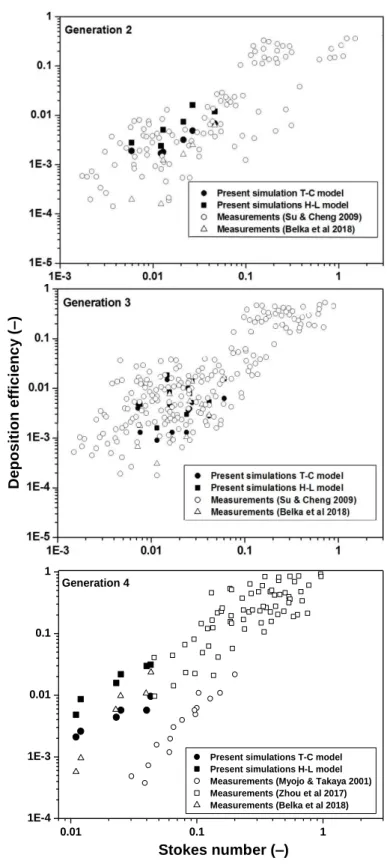
An even better matching of the numerical and experimental results could be observed in airway generations 2 – 4 depicted in Figure 9.
Figure 9. Simulated deposition efficiency of fibres (filled symbols) in the second (upper panel), third (middle panel) and fourth (lower panel) airway generations as a function of Stokes number in comparison with the experimentally measured values (empty symbols)
Stokes number (–)
Deposition efficiency (–)
0.01 0.1 1
1E-4 1E-3 0.01 0.1 1
Generation 4
Deposition efficiency (-)
Stokes number (-)
Present simulations T-C model Present simulations H-L model Measurements (Myojo & Takaya 2001) Measurements (Zhou et al 2017) Measurements (Belka et al 2018)
23
In agreement with the notations in Belka et al (2018), there were two second generation airway segments (segments 5 and 8), four third generation segments (segments 6, 7, 9 and 10) and two fourth generation segments (segments 11 and 12) considered (see Figure 4). The other fourth generation airways were not segmented separately, but they were parts of multigenerational segments. Therefore, it was assumed that the two fourth generation segments represent all the bifurcations in the fourth generation. The good match between the measured and computed deposition efficiency values indicates that the numerical models described in the Methods section reasonably simulate the real case of fibre deposition in the large human airway bifurcations for which experimental data is available.
Obviously, the models defined and presented in this paper can be improved from several aspects. For instance, it has been specified in the work of Tran-Cong et al (2004) that equation (8) is valid for particle Reynolds numbers between 0.15 and 1500. For the present fibre dimensions and air velocity values in the airways theoretically it is not realistic to exceed the upper limit. The fulfilment of this condition was verified after the simulations. However, for very low Reynolds numbers a correction may be applied. As mentioned before, the applied turbulent dispersion model is also suboptimal and a near-wall correction could be implemented in the future to improve the accuracy of numerical predictions, especially in the upper airways.
In addition, it has been assumed in the present paper that any fibre touching the wall of the airways deposits at that location. In reality, the probability of deposition may be a function of the impaction angle. Most probably, deposition has higher chances if the fibre forms an angle with the airway surface close to zero degrees and deposition is less probable if the angle is around 90 degrees. Systematic experiments aiming at the quantification of deposition as a function of contact angle and inclusion of the results into numerical models could further improve the quality of deposition simulations. Last but not least, fibre orientation was randomly selected in this work. The primary aim of this early research paper was to compare the available experimental data with the results of CFD modelling assuming equal chances for any orientation. One of the main conclusions is that based on the results as realistic as possible probability functions are needed in the future to improve the accuracy of the computations. Our next step will be to apply probability functions deduced for straight tubes and symmetric bifurcations and verify the effect of the introduction of weighted orientations. These developments may lead to a more realistic tracking of fibre orientation.
24 4. Conclusions
Mutually validated numerical simulations and experimental measurements can provide an appropriate fibre dosimetry in different parts of the airways. Present study has demonstrated that carefully implemented complex numerical models can be powerful tools in characterizing the efficiency of different airway segments to filter the inhaled fibres. Our simulation results were generally in line with the available experimental measurement results of Su and Cheng (2005), Su and Cheng (2009) and Belka et al (2018). The main outcome of the current computations was that most of the fibres penetrate into the deeper regions of the airways, where mucociliary clearance is not so effective or does not exist. To what extent macrophages from the deep airways cope better with glass fibres than with asbestos, remains to be established.
Current work also highlighted the importance of using physically more realistic drag models, taking into account not only the deviation from spherical shape (sphericity), but also the dimensional anisotropy (aspect ratio) and orientation of fibres.
Acknowledgement
This work was supported by the CZ.02.2.69/0.0/0.0/16_027/0008371 project, the Czech Science Foundation grant GA18-25618S and the Project of the Czech National Programme INTER-COST, LTC17087, as a part of the COST Action SimInhale.
The authors would like to thank Dr Miloslav Belka for providing his experimental data for comparison with the results of numerical simulations.
References
Balásházy, I., Hofmann, W., & Heistracher, T. (2003). Local particle deposition patterns may play a key role in the development of lung cancer. Journal of Applied Physiology, 94, 1719–
1725.
Balásházy, I., Moustafa, M., Hofmann, W., Szőke, R., El-Hussein, A., & Ahmed, A-R. (2005).
Simulation of fibre deposition in bronchial airways. Inhalation Toxicology, 17, 717–727.
Barbieri, P. G., Mirabelli, D., Somigliana, A., Cavone, D., & Merler, E. (2012). Asbestos fibre burden in lungs of patients with mesothelioma who lived near asbestos-cement factories.
Annals of Occupational Hygiene, 56, 660–670.
Baron, P. A., & Willeke, K. (2001). Aerosol measurement: Principles, techniques and Application (2nd ed.). New York: Wiley.
Belka, M., Lizal, F., Jedelsky, J., Elcner, J., Hopke, P. K., & Jicha, M. (2018). Deposition of glass fibers in a physically realistic replica of the human respiratory tract. Journal of Aerosol Science, 117,149–163.
25
Bernstein, D., Dunnigan, J., Hesterberg, T., Brown, R., Velasco, J. A. L., Barrera, R., Hoskins, J., & Gibbs, A. (2013). Health risks of chrysolite revisited. Critical Reviews in Toxicology, 43, 154–183.
Cai, F. S., & Yu, C. P. (1988). Inertial and interseptional deposition pf spherical particles and fibres in a bifurcating airway. Journal of Aerosol Science, 19, 679–688.
Cheng, K. H., Cheng, Y. S., Yeh, H. C., & Swift, D. L. (1997) Measurements of airway dimensions and calculation of mass transfer characteristics of the human oral passage. Journal of Biomechanical Engineering-Transactions of the ASME, 119, 476–482.
Dastan, A., Abouali, O., & Ahmadi, G. (2014). CFD simulation of total and regional fiber deposition in human nasal cavities. Journal of Aerosol Science, 69, 132–149.
Debhi, A. (2011). Prediction of extrathoracic aerosol deposition using RANS-random walk and LES approaches. Aerosol Science and Technology, 45, 555–569.
Elcner, J., Lizal, F., Jedelsky, J., Jicha, M., & Chovancova, M. (2016). Numerical investigation of inspiratory airflow in a realistic model of the human tracheobronchial airways and a comparison with experimental results. Biomechanics and Modelling in Mechanobiology, 15, 447–469.
Farkas, Á., Balásházy, I., & Szőcs, K. (2006). Characterization of regional and local deposition of inhaled aerosol drugs in the respiratory system by computational fluid and particle dynamics methods. Journal of Aerosol Medicine, 19, 329–343.
Farkas, Á., Horváth, A., Kerekes, A., Nagy, A., Kugler, Sz., Tamási, L., & Tomisa, G. (2018).
Effect of delayed pMDI actuation on the lung deposition of a fixed-dose combination drug.
International Journal of Pharmaceutics, 547, 480–488.
Feng, Y., & Kleinstreuer, C. (2013). Analysis of non-spherical particle transport in complex internal shear flows. Physics of Fluids, 25, 091904-1–0.91904-26.
Fuchs, N. A. (1964). The mechanics of aerosols. Oxford: Pergamon Press.
Ganser, G. H. (1993). A rational approach to drag prediction of spherical and non-spherical particles. Powder Technology, 77, 143–152.
Garland, L. H. (1961). Bronchial carcinoma. Lobar distribution of lesions in 250 cases.
California Medicine, 94, 7-8.
Gonda, I., Abd El Khalik, A. F. (1985). On the calculation of aerodynamic diameters of fibers.
Aerosol Science and Technology, 4, 233–238.
Haider, A., & Levenspiel, O. (1989). Drag coefficient and terminal velocity of spherical and nonspherical particles. Powder Technology, 58, 63–70.
Harris, R.L., & Fraser, D. A. (1976). A model for deposition of fibres in the human respiratory system. American Industrial Hygiene Association Journal, 37, 73–89.
Hartmann, M., Trnka, O., & Svoboda, K. (1994). Free settling of nonspherical particles.
Industrial and Engineering Chemistry Research, 33, 1979–1983.
26
IARC International Agency for Research in Cancer (2002). Working Group on the Evaluation of Carcinogenic Risks to Humans. World Health Organization. Man-made vitreous fibres, Lyon, France.
Inthawong, K., Wen, J., Tian, Z., &Tu, J. (2008). Numerical study of fibre deposition in a human nasal cavity. Journal of Aerosol Science, 39, 253–265.
Inthawong, K., Mouritz, A. P., Dong, J., & Tu, J. Y. (2013). Inhalation and deposition of carbon and glass composite fibre in the respiratory airways. Journal of Aerosol Science, 65, 58–68.
Jeffery, G. B. (1922). The motion of ellipsoidal particles immersed in in a viscous fluid.
Proceedings of the Royal Society of London A: Mathematical, Physical and Engineering Sciences, 102, 161–179.
Koullapis, P., Kassinos, S. C., Muela, J., Perez-Segarra, C., Rigola, J., Lehmkuhl, O., Cui, Y., Sommerfeld, M., Elcner, J., Jicha, M., Saveljic, I., Filipovic, N., Lizal, F., & Nicolaou, L.
Regional aerosol deposition in the human airways: The SimInhale benchmark case and the critical assessment of in silico methods. European Journal of Pharmaceutical Sciences, 113, 77–94.
Lizal, F., Elcner, J., Hopke, P. K., Jedelsky, J., & Jicha, M. (2012). Development of a realistic human airway model. Proceedings of the Institution of Mechanical Engineers Part H-Journal of Engineering in Medicine, 226, 197–207.
Lizal, F., Belka, M., Adam, J., Jedelsky, J., & Jicha, M. (2015). A method for in vitro aerosol deposition measurement in a model of the human tracheobronchial tree by the positron emission tomography. Journal of Engineering in Medicine, 229, 750–757.
Myojo, T. (1990). The effect of length and diameter on the deposition of fibrous aerosol in a model bifurcation. Journal of Aerosol Science, 21, 651–659.
Myojo, T., Takaya, M. (2001). Estimation of fibrous aerosol deposition in upper bonchi based on experimental data with model bifurcation. Industrial Health, 39, 141–149.
Prodi, V., De Zaiacomo, T., Hochrainer, D., & Spurny, K. (1982). Fibre collection and measurement with the inertial spectrometer. Journal of Aerosol Science, 13, 49–58.
Schmidt, A., Zidowitz, S., Kriete, A., Denhard, T., Krass, S., & Peitgen, H. O. (2004). A digital reference model of the bronchial tree. Computerized Medical Imaging and Graphics, 28, 203–
211.
SCOEL Scientific Committee on Occupational Exposure Limits (2012). Recommendation of the Scientific Committee on Occupational Exposure Limits for man-made mineral fibres (MMMF): European Commission, Employment, Social Affairs and Inclusion.
Shukla, A., Gulumian, M., Hei, T. K., Kamp, D., Rahman, Q., & Mossman, B. T. (2003).
Multiple roles of oxidants in the pathogenesis of asbestos-induced diseases. Free Radical Biology and Medicine, 34,1117–1129.
Stöber, W. (1972). Dynamic shape factors of nonspherical aerosol particles. In: Assessment of airborne particles. (ed. Mercer, T. T., Morrow, P. E., & Stöber, W.), 249–288, Springfield.
27
Su, W. C., & Cheng, Y. S. (2005). Deposition of fibre in the human nasal airway. Aerosol Science and Technology, 39, 888–901.
Su, W. C., & Cheng, Y. S. (2009). Deposition of man-made fibers in human respiratory airway casts. Journal of Aerosol Science, 40, 270–284.
Sussman, R. G., Cohen, B. S., & Lippmann, M. (1991). Asbestos fiber deposition in a human tracheobronchial cast. I. Experimental. Inhalation Toxicology, 3, 145–160.
Tian, L., Ahmadi, G. (2013). Fiber transport and deposition in human upper tracheobronchial airways. Journal of Aerosol Science, 60, 1–20.
Tran-Cong, S., Gay, M., & Michaelides, E. E. (2004). Drag coefficients of irregularly shaped particles. Powder Technology, 139, 21–32.
Veeze, P. (1968). Rationale and methods of early detection in lung cancer. Van Gorcum, Assen, The Netherlands.
Wang, Z., Hopke, P. K., Ahmadi, G., Cheng, Y. S., & Baron, P. A. (2008). Fibrous particle deposition in human nasal passage: The influence of particle length, flow rate, and geometry of nasal airway. Journal of Aerosol Science, 39, 1040–1054.
White, F. M. (2011). Fluid Mechanics (7th ed.). New York: McGraw Hill.
Wadell, H. (1933). Sphericity and roundness of rock particles. Journal of Geology, 41, 310–
331.
Zhou, Y., Su, W. C., & Cheng, Y. S. (2007). Fiber deposition in the tracheobronchial region:
Experimental measurements. Inhalation Toxicology, 13, 109–127.
Zhang, L., Asgharian, B., & Anjivel, S. (1996). Inertial and inteceptional deposition of fibers in a bifurcating airway. Journal of Aerosol Medicine, 9, 419–429.