Journal of Aerosol Science 150 (2020) 105649
Available online 28 August 2020
0021-8502/© 2020 Elsevier Ltd. All rights reserved.
The effect of oral and nasal breathing on the deposition of inhaled particles in upper and tracheobronchial airways
Frantisek Lizal
a,*, Jakub Elcner
a, Jan Jedelsky
a, Milan Maly
a, Miroslav Jicha
a, Arp ´ ´ ad Farkas
a,b, Miloslav Belka
a, Zdenek Rehak
c, Jan Adam
c,d, Adam Brinek
e, Jakub Laznovsky
e, Tomas Zikmund
e, Jozef Kaiser
eaBrno University of Technology, Faculty of Mechanical Engineering, Energy Institute, Technicka 2896/2, Brno, 616 69, Czech Republic
bCentre for Energy Research, Konkoly-Thege Mikl´os u. 29-33, 1121, Budapest, Hungary
cMasaryk Memorial Cancer Institute, Zluty kopec 7, Brno, 602 00, Czech Republic
dÚJV ˇReˇz, a.s., Hlavni 130, Husinec-Rez, Rez 250 68, Czech Republic
eCEITEC - Central European Institute of Technology, Brno University of Technology, Purkynova 123, Brno, 612 00, Czech Republic
A R T I C L E I N F O Keywords:
Computational fluid mechanics Numerical simulations Particle deposition Positron emission tomography Laser Doppler anemometry Flow
Airways Lungs
Deposition hotspots
A B S T R A C T
The inhalation route has a substantial influence on the fate of inhaled particles. An outbreak of infectious diseases such as COVID-19, influenza or tuberculosis depends on the site of deposition of the inhaled pathogens. But the knowledge of respiratory deposition is important also for occupational safety or targeted delivery of inhaled pharmaceuticals.
Simulations utilizing computational fluid dynamics are becoming available to a wide spectrum of users and they can undoubtedly bring detailed predictions of regional deposition of particles.
However, if those simulations are to be trusted, they must be validated by experimental data. This article presents simulations and experiments performed on a geometry of airways which is available to other users and thus those results can be used for intercomparison between different research groups. In particular, three hypotheses were tested. First: Oral breathing and combined breathing are equivalent in terms of particle deposition in TB airways, as the pressure resistance of the nasal cavity is so high that the inhaled aerosol flows mostly through the oral cavity in both cases. Second: The influence of the inhalation route (nasal, oral or combined) on the regional distribution of the deposited particles downstream of the trachea is negligible. Third: Simulations can accurately and credibly predict deposition hotspots. The maximum spatial resolution of predicted deposition achievable by current methods was searched for. The simulations were performed using large-eddy simulation, the flow measurements were done by laser Doppler anemometry and the deposition has been measured by positron emission tomography in a real- istic replica of human airways. Limitations and sources of uncertainties of the experimental methods were identified.
The results confirmed that the high-pressure resistance of the nasal cavity leads to practically identical velocity profiles, even above the glottis for the mouth, and combined mouth and nose breathing. The distribution of deposited particles downstream of the trachea was not influenced by the inhalation route. The carina of the first bifurcation was not among the main deposition hotspots regardless of the inhalation route or flow rate. On the other hand, the deposition
* Corresponding author.
E-mail address: lizal@fme.vutbr.cz (F. Lizal).
Contents lists available at ScienceDirect
Journal of Aerosol Science
journal homepage: http://www.elsevier.com/locate/jaerosci
https://doi.org/10.1016/j.jaerosci.2020.105649
Received 8 April 2020; Received in revised form 5 August 2020; Accepted 13 August 2020
Journal of Aerosol Science 150 (2020) 105649 hotspots were identified by both CFD and experiments in the second bifurcation in both lungs, and to a lesser extent also in both the third bifurcations in the left lung.
1. Introduction
Spreading of infectious diseases such as influenza, tuberculosis or COVID-19 (novel coronavirus SARS-CoV-2) depends on the inhalation of aerosolized pathogens. The transmission of the disease involves several factors: the type and frequency of respiratory activity, the concentration of particles loaded with pathogens, the type of pathogen and the site of infection (Gralton, Tovey, McLaws,
& Rawlinson, 2011). It is well known that an outbreak of a disease and its severity depends strongly on the site where the inhaled
pathogens deposit within the human airways. When infectious germs reach lower respiratory tract, they represent a high risk and are associated with higher morbidity and fatality (Fendrick, Monto, Nightengale, & Sarnes, 2003; Gralton et al., 2011) compared with upper airway infections.
The demand for accurate prediction of the deposition site of inhaled particles is of course not limited to bioaerosols but is vital for protection against all types of harmful pollutants, and for targeted delivery of pharmaceuticals. In general, due to various occupations and physical exertion that people are submitted to in both indoor and outdoor environment, different breathing patterns are activated and thus the aerosol penetrates the respiratory tract essentially by two routes: either by the nasal or oral route separately, or by both, depending on physical activities and whether the aerosol is environmental or pharmaceutical (for example pharmaceutical aerosols are typically delivered through oral inhalation which is considered superior to the nasal route in adults).
Aerosol inhalation in infants and toddlers is significantly different from that of adults. As stated by Amirav, Borojeni, Halamish, Newhouse, and Golshahi (2015), up to the age of 20 months the nasal breathing exceeds that of oral breathing and becomes equivalent just at the age of 20 months. This is due to different development stages of nasal and oral cavities in the early ages. For example, the oro-pharyngeal passages in infants appear somewhat more convoluted than the nasopharyngeal airways and the nasopharyngeal angle is much less acute than in the adults. The study has shown, that the nasal inhalation is more efficient for aerosol delivery to the lower airways than mouth inhalation in infants and toddlers.
The importance of nasal passage geometry was proved by Bennett and Zeman (2005) who studied the effect of race on fine particle deposition for oral and nasal breathing. They concluded that compared with Caucasian (C) adults, African-American (AA) adults have reduced nasal efficiency in association with lower nasal resistance and less elliptical nostrils in AA subjects. Consequently, the AA subjects appear to have less efficient nasal filtration of fine particles.
Besides the inherent differences between the breathing modes (oral versus nasal) of infant and adult subjects and the significant ethnic group-specific variabilities among the adult population, the inhalation route depends also on airway health status. There are certain health conditions when people prefer the oral inhalation route because of a temporary (e.g. flu, allergy) or permanent (e.g.
deviated septum or small nostril size) partial or total unavailability of the nasal route (mouth breathers, ICRP (1994)). Finally, the inhalation route can be deliberately influenced by the individual. For instance, it is recommended to breathe through the nose in places with high pollution or infection risk, since the nose is (generally) a better filter than the mouth (see below). Also, clearance is more effective there and the underlying cells are less sensitive than those in the deep lungs.
Heyder, Armbruster, Gebhart, Grein, and Stahlhofen (1975) tested five volunteers who breathed either through a tube in the mouth or through an airtight nose mask. They concluded that deposition is quite different when breathing through the nose. Total deposition depends not only on the flow rate but also on the varying breathing frequency with constant tidal volume. For high flow rates, the difference between the nose and mouth breathing is remarkable, whereas for low flow rates it is much less pronounced, due to deposition in the nasal passages. As also stated by Horschler, Brucker, Schroder, and Meinke (2006), the shape of the nasal cavity has a paramount impact on the aerodynamics of the flow and thus plays a crucial role in the nasal deposition as a fraction of the whole lungs deposition.
Everard, Hardy, and Milner (1993) confirmed that the penetration of aerosol into the lung is greatly reduced when breathing through the nose compared with mouth breathing. The mean increase in lung deposition (calculated as a percentage of the whole body deposition) when breathing through the mouth was 37%. However, the distribution of deposited particles among the central, mid, and peripheral regions when expressed as a percentage of the dose deposited in the lungs was almost identical for both routes. But would the distribution be identical if we had focused in individual branches? Would there be deposition hotspots formed in identical locations?
The current question when assessing the nasal or oral breathing and its effect on aerosol delivery to the lungs is not whether the former or latter is better from the perspective of aerosol deposition efficiency, but how exactly is the deposition of aerosols in the lower branches of the tracheobronchial (TB) tree different if administered nasally or orally and whether there is a significant difference in the distribution of deposited conventional aerosols among the specific branches and generations of airways, or whether deposition hot- spots are formed for either of the breathing routes. In other words, if there might be differences in local deposition patterns which may result in an outbreak of infectious diseases in different regions of lower airways among mouth or nose breathers.
As mentioned above, both routes for the delivery of aerosols are used and which one prevails depends on the situation and physical F. Lizal et al.
conditions. The nose breathing and aerosol delivery may be considered more frequent in low physical activities and in small children as stated above. Tian, Hindle, and Longest (2014) conclude with surprising finding (in the light of the previously mentioned articles), that nose-lung TB tree delivery with a conventional1 aerosol performed comparably to orally inhaled products. However, a potential disadvantage of nose-to-lung delivery with conventional sized aerosols is the exposure of the nose to high concentrations of the aerosol.
For prediction of the flow field and aerosol deposition, simulations using Computational Fluid Dynamics (CFD) approach are frequently used. The CFD approach, also called in-silico, enables to account for detailed structures of the flow field, for example, flow separation and secondary flow in curved airways. Numerous papers deal with the TB aerosol deposition through the oral or nasal passages. Most papers have studied aerosol deposition through the oral administration, see for example a very complex review of in- silico methods by Koullapis, Kassinos et al. (2018). A similar paper by Koullapis, Nicolaou, and Kassinos (2018) studied the influence of different mouth-throat geometries on the deposition in the lower generations of the TB tree and concluded that there is no difference in the deposition, thus claiming that extrathoracic regions can be excluded while performing simulations in the lower generations of the TB tree in order to reduce time needed for the simulations. They considered an airway geometry consisting of oral passages, pharynx, larynx, trachea and large bronchi. Since the nasal airways were not considered, this study did not analyse the consequences of switching to nasal or combined breathing. The present study can be seen as an extension of their work by adding the nasal airways (because their geometry and our geometry are identical with the exception of the newly added nasal cavity) and measuring and simulating the complex airflows and deposition patterns assuming different breathing modes (oral, nasal, combined).
The nasal cavity due to its geometric complexity plays a more significant role than the oral cavity in the airflow at the pharynx/
larynx region where high turbulence intensity (TI) is generated. In the paper by Ghahramani, Abouali, Emdad, and Ahmadi (2014), dispersion of micro-particles in the human airway from nostrils to the end of the trachea was studied. The flow field was modelled using Low Reynolds Number (LRN) k-ε model, which is shown here to be superior to LRN k-ω model not only for the prediction of mean flow velocities but also for the turbulence kinetic energy. Concerning the particles deposition, application of the Continuous Random Walk (CRW) model in contrast with the classical Discrete Random Walk by Gosman and Ioannides (1981), which overpredicts the deposition, provides a better agreement with experiments published by Kelly, Asgharian, Kimbell, and Wong (2004a). Ghahramani et al. (2014) also concluded that in the turbulent regime no particles with the diameter >10 μm can enter the lung unlike in laminar flow at rest.
Although several papers on comparison between the nasal and oral administration have been published in the past, we believe that systematic comparison involving both experiments and simulations is needed. In the paper by Zhang and Kleinstreuer (2011), a study of airflow and aerosol deposition penetrating by both routes was carried out for nanoparticles smaller than 40 nm. The study shows that airflow at the pharynx/larynx region under simultaneous nasal and oral inhalation exhibits significant differences when compared with nasal or oral breathing only. The nasal-to-oral flow rate ratio has a large effect on nanoparticle deposition in the regions of pharynx, larynx and trachea, and even at main bronchi bifurcations, especially for particles with diameters less than 5 nm. In contrast, the change of breathing route has only a minor effect on nanoparticle deposition at and beyond the larynx region for particles larger than 5 nm. However, the ratio of the nasal and oral flow rate was “artificially” adjusted to different values, and thus we do not know what could be the flow distribution when the mouth is fully open and the oral and nasal flow rates develop as a result of hydraulic resistances of both routes. The deposition results of Zhang and Kleinstreuer were not underpinned by in vitro experimental mea- surements in the same geometry assuming similar breathing conditions. On the contrary, in the present work both in vitro and in silico results are presented.
In the earlier study, Subramaniam, Richardson, Morgan, Kimbell, and Guilmette (1998) applied CFD techniques to explore the complexity of the airflow in the nasal passages. Their airway geometry did not contain the oral cavity nor bronchi. Their work did not include experimental measurements. Moreover, in their work Subramaniam et al. focused exclusively on the flow field and did not study the transport of inhaled particles.
Phuong and Ito (2015) investigated flow pattern in the trachea for oral and nasal inhalation with a constant flow rate of 7.5, 15 and 30 L/min in a realistic but simplified respiratory tract acquired from CT scan. Mean velocities were presented in three different tracheal cross-sections for oral and nasal breathing with no deep analysis of differences for the two administration routes. However, as could be seen from several graphs, it seems that there is a larger separation region for the nasal breathing than for the oral breathing in the posterior side of the trachea downstream of the larynx. This could lead to different particle deposition but needs to be proven by further studies. One of the goals of our study is to bring this missing piece of information on particle deposition.
The importance of studying the influence of the upper airway structures on the flow has been emphasized by Lin, Tawhai, McLennan, and Hoffman (2007) who found that “the presence of turbulence in the subglottic space increases the localised tracheal wall shear stress by three folds. The study also shows that neglecting the oropharynx and larynx leads to different flow structures: velocity parabola in the trachea and negligible turbulence”. In summary of their work they concluded: “The comparison of flow characteristics in models that include or neglect the mouth–oropharynx–larynx suggest that simple inlet boundary conditions do not adequately represent the effect of the upper airway structures, affecting the estimate of flow through several generations of the airway and the tracheal wall shear stress.”
It must be emphasized, that although the CFD simulations are widely believed to bring detailed understanding to the flow and deposition of particles and could potentially be used in patient-tailored medicine, the confidence in the simulated results is not a matter of course. In general, CFD simulations should be validated with the experimental data, preferably on a geometry identical with the
1 In contrast with enhanced condensational growth aerosol when the particles increase their sizes on the upper airways due to contact with wet airways environment.
Journal of Aerosol Science 150 (2020) 105649 calculations. In this paper, we present such CFD calculations of airflow and deposition of inhaled particles validated with experimental data. The airflow has been validated by laser Doppler anemometry (LDA) and the deposition by positron emission tomography (PET).
PET is one of the common methods of medical imaging, routinely used as a non-invasive method of diagnostics, in several fields of medicine, primarily oncology, cardiology and neurology. The method is based on the administration of a pharmaceutical containing a radionuclide undergoing beta-plus decay and emitting a positron. The crucial step is the detection of photons simultaneously emitted by a positron-electron annihilation, which occurs almost immediately after the positron emergence.
The above presented state-of-the-art documents the current knowledge of the influence of the inhalation route on the lung flow. Our aim was to focus more deeply on this issue, to simulate and measure the inhalation through the nose, mouth or both and see its effect not only on the flow but also on the deposition of particles in a realistic TB geometry.
The medical community seeks for more detailed prediction of aerosol deposition (see e.g. (Hofmann, 2011)). The evidence that local accumulation of inhaled particles causes the development of carcinoma has been collected e.g. by Churg and Vedal (1996). The accumulation of inhomogeneous high concentration of inhaled particles has been reported very recently by (Mekonnen, Cheng, &
Kourmatzis, 2020). Hence, limits of the current technology as regards precision and maximal achievable resolution for prediction and measurement of regional deposition in upper and TB airways were searched for.
Several hypotheses were formulated and tested
First: Oral breathing and combined breathing are equivalent in terms of particle deposition in TB airways, as the pressure resistance of the nasal cavity is so high that most of the inhaled aerosol flows through the oral cavity in both cases.
Second: The influence of the inhalation route (nasal, oral or combined) on the regional distribution of the deposited particles downstream of the trachea is negligible.
Third: Simulations can accurately and credibly predict deposition hotspots.
For brevity, the inhalation through the nose with a closed mouth is abbreviated as NB, mouth breathing is denoted as MB and the
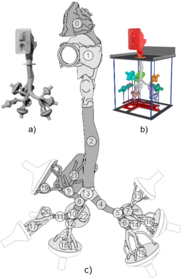
Fig. 1.Visualization of the airway replica for deposition (a) and flow (b) measurements, and a scheme of the segment numbers (c). The face mask is not depicted.
F. Lizal et al.
combined inhalation through both nose and mouth is referred to as CB.
2. Methods
As the determination of the maximal achievable resolution when predicting the deposition hotspots was one of the goals of this study, the application of identical airway geometry for simulations and experiments was a must. The preparation of the computational mesh and the physical replicas of airways, as well as the numerical and experimental setup, are reported in the following section.
2.1. The digital geometry of the airways
The geometry of airways used for this study is based on the lung model developed at Brno University of Technology for a long time (Lizal, Elcner, Hopke, Jedelsky, & Jicha, 2012). This geometry originally consisted of the oral cavity, larynx and TB tree down to the seventh generation of branching. As the current study aimed to compare the airflow and deposition during nasal, oral and combined breathing, an existing geometry had to be extended with a nasal cavity. Its geometry was acquired from the University of California Davis (Sarangapani & Wexler, 2000) as a stereolithographic (STL) file created from original computed tomography scans of the nasal cavity of a healthy 25-year old male. The STL geometry contained all paranasal sinuses and protuberances and therefore it needed to be adjusted to create digital geometry suitable for both CFD simulations and fabrication of physical airway replicas. Sinuses, unwanted for this study, were cleared using commercial computer-aided design program Rhinoceros 3D (McNeel, Seattle, WA 98103 USA), and the whole topology of the model was then smoothed using a module for creating and editing surface meshes in Star-CCM+(CD-adapco, Melville, NY, USA) to remove the unwanted fragments which the original coarse geometry contained.
The nasal cavity was then connected to the oral cavity from the original model. This connection was done with respect to the available literature (Putz & Pabst, 2007) and after several consultations with experienced otorhinolaryngologist. The aim of the consultations was to find the correct size ratio of the nasal and oral cavity, the proper position of the nasal cavity to the rest of the airways, and the shape accuracy of the nasopharynx and the soft palate, which were completely modelled. The nasal cavity surface area is 13 482 mm2; the volume is 9771 mm3. The resulting composite geometry of human upper respiratory tract segmented for purposes of deposition study can be seen in Fig. 1.
In the second stage of work, the digital geometry was adjusted to satisfy the requirements of the LDA for measurements of flow velocity (Fig. 1b) and PET for measurements of particle deposition (Fig. 1a). To ensure the realistic velocity field at the inlet of the geometry, it was decided to shape the exterior of the model in a face-like manner. The simplified mouth has a circular cross-section of 20 mm, which corresponds to the inlet of the former airway replica that contained only the oral cavity. The internal shape of the geometry was not modified. The lengths, diameters and branching angles of the TB tree have been reported in (Lizal et al., 2012). The specific adjustments of the digital geometry in order to provide the CFD mesh and for production of the replicas used for measurements are described in the following paragraphs.
2.2. Setup of numerical simulations 2.2.1. The computational mesh
An unstructured hybrid numerical mesh with polyhedral core elements and prismatic boundary layer was generated on the three considered geometries (MB, NB, CB). They differ from each other only at the level of nasal and oral entrances; hence, the corresponding meshes were quite similar. The base size of the grid element was set on the basis of maximal assumed airflow through the models (60 L/
min). The base size had to fulfil the Taylor microscale criterion because the calculations were performed by the use of a large-eddy model. Accordingly, the base size was set to 0.5 mm. A prismatic layer, consisting of ten layers of cells with increasing cell size from the wall to the core of the model, was also generated to properly describe the flow in the near-wall boundary layer. The thickness of the whole prismatic layer was 0.5 mm and the thickness of the first near-wall cell layer was set to 0.02 mm to comply with the y+<1 condition (y+-non-dimensional wall distance) enabling us to resolve the effects in the viscous near-wall sublayer. Since the value of y+can be only estimated prior to the simulations, the exact values were checked after the simulations to make sure that the y+<1 condition for the height of the first cells was indeed satisfied. The independence of the results of numerical simulations from the generated mesh was tested by comparing the results achieved on meshes with different resolutions (6, 10, 14 and 18 million cells) for the flowrate of 60 L/min. The mesh test demonstrated that the mesh with 14 million cells provided the best compromise between accuracy and computational demands. The particularities of the mesh generated on the geometry used to simulate mouth breathing can be seen in Fig. 2.
The digital geometry and the computational mesh is available to any research group for non-profit purposes upon request by the authors of this article. The original airway geometry without the nasal cavity can be downloaded from the Ercoftac database (P.
Koullapis et al., 2019).
The numerical simulations were performed by the Star-CCM+commercial solver (version v10.04.011, CD-adapco, Melville, NY, USA). The unsteady velocity field was calculated by a segregated solver with bounded central-differencing convection scheme and the SIMPLE algorithm was applied for pressure-velocity coupling. A pressure boundary condition with zero pressure resistance was prescribed at the inlet tube of the mask and uniform air velocity values were prescribed at each of the ten outlets according to experimentally measured values (see Table 1). The turbulence intensity was not prescribed at the inlet, but it has been generated by the flow in the mask. In other words, the face mask served as entrance, flow conditioning section. The process of generation of fluctuations in the mask and replica can be observed in Figs. A4 and A8 in Appendix A. It can be seen that most fluctuations were generated at
Journal of Aerosol Science 150 (2020) 105649
nostrils and mouth inlet. However, the possible influence of the inflow turbulence generation techniques will be studied in the future.
Turbulence was modelled using a large-eddy simulation (LES) approach with wall adapting local eddy (WALE) viscosity subgrid- scale model activated. The constants of the WALE model were Cw =0.544, Ct =3.5 and κ =0.41. The time step was 5.0⋅10−5 s and ten internal iterations were performed during each time step. The average value of the Courant number in all cells during the calculation was 0.32. Less than 0.01% of the cells had Courant number C >5.
The simulation started with a steady RANS pre-calculation of the initial velocity field using SST k-ω turbulence model. After the pre- calculation, it was switched to the unsteady LES. The instantaneous velocity was monitored in six selected points of the geometry (the mouth cavity, larynx, trachea above the bifurcation, and 1st, 2nd and 3rd generation of branching) before initiation of the averaging of the velocity. Stabilisation of the velocity fluctuations around a constant velocity value was observed after approx. 0.3 s of the LES calculation. The averaging of velocity values started from the time 1.1 s after the beginning of the LES simulation. Instantaneous velocity has been recorded every time-step and all instantaneous velocity magnitude values were used for calculation of mean velocity magnitude. The averaging period was 1 s. Care has been taken to ensure that the time used for the averaging of the solution is Fig. 2.Details of the computational mesh generated on model geometry. The number in each respective cross-section indicates the used ampli- fication factor. Settings of the flow simulations.
Table 1
Flowrates and surface areas of specific segments of the airway replica.
Segment ID Flow rate (L/min) Airway generation Surface area (cm2)
0 30 60 Nasal cavity 144.1
1 Oral cavity 146.2
2 30 60 G0 - trachea 60.2
3 30 60 G1 9.7
4 8.9 17.8 G1 9.2
5 8.9 17.8 G2 3.6
6 5.6 11.2 G3 5.7
7 3.3 6.6 G3 4.0
8 21.1 42.2 G2 8.6
9 6.9 13.8 G3 6.0
10 14.3 28.6 G3 4.9
11 6.7 13.4 G4 6.1
12 7.6 15.2 G4 4.1
13 1.4 2.8 G4–G6 10.1
14 1.6 3.2 G4–G6 16.1
15 4.0 8 G4–G7 25.2
16 1.9 3.8 G4–G6 10.7
17 3.6 7.2 G5–G6 14.4
18 4.7 9.4 G5–G7 17.7
19 3.8 7.6 G4–G6 21.9
20 3.1 6.2 G4–G6 5.9
21 3.1 6.2 G4–G6 21.0
22 3.0 6 G5–G6 10.6
Total inspiratory flow rate (L/min) 30 60
F. Lizal et al.
sufficiently long to produce the mean solution that is not a function of time. The actual averaging period represented approx. 7 times the mean flow residence time in the solution domain (L/v =0.14 s, where L is the characteristic length of the solution domain estimated as a distance from the mouth inlet to the outlet of segment 28, and v is the characteristic mean flow velocity determined as an average of mean velocities in replica calculated from the flowrate and tube diameter of the respective airway segments).
In the case of large-eddy simulations, only the large energetic scales are resolved. The small unresolved scales are modelled using a subgrid-scale model. In this work, we have applied the WALE model, which alleviates the most severe deficiencies of Smagorinsky model such as wall proximity behaviour of the eddy-viscosity and the laminar to turbulence transition. Although this model proved to be appropriate in several applications, it is not lacking errors, thus both the mean velocity and the fluctuating velocity are prone to error. The two main sources of errors are the modelling errors due to filtering, subgrid-scale and boundary conditions and the dis- cretisation errors due to the numerical schemes. It was previously demonstrated, e.g. (Lang & Teleaga, 2008), that for certain ranges of filter width (approximately equal to the grid size) the two types of errors interact and that discretisation errors can be equal or even higher than the subgrid modelling terms (Ghosal, 1996). The default choice of the length scale built-in the Star CCM+had been suited to minimize the error and hence was not modified in our study.
2.2.2. Settings of the particle deposition simulations
The Lagrangian multiphase model was used to simulate particle transport and deposition in the studied airways. To quantify the aerosol deposition, 100 000 particles were injected into the model. The particles were released after 1.1 s of LES calculation when the flow was fully developed. There were 100 injection points equally distributed over the inlet of the face mask. Ten particles were injected during each time-step from each injection point during the first 100 time-steps. In total, 100 000 particles were injected within 5 ×10⁻³ s. It is worth noting that the injection – inhalation time plays an important role, and if all the particles had entered the replica at once, they would have been influenced by fluctuations of the flow which might result in distorted deposition pattern. In our case, the face mask again served as an entrance reservoir, where the particles were subjected to the whirling flow, some of them were delayed, and they entered the replica within a time window of approx. 0.7 s. The visualization of the inhalation can be seen in the supple- mentary file.2
Supplementary video related to this article can be found at https://doi.org/10.1016/j.jaerosci.2020.105649
The particles were non-interacting, and one-way coupling between the airflow and particles was considered. This means that the fate of the inhaled particles was influenced by the airflow stream, but the particles did not affect the flow. The particles were tracked by numerical integration of their force balance equation. The drag force, gravity and pressure gradient forces were considered to act on the particles. Particle characteristics were set according to the experimentally measured values. Since DEHS (di-2-ethyl-hexyl-seba- cate) particles were considered, the density of 912 kg/m3 was set and the size of particles was prescribed using cumulative distribution tables, which were derived from experimental size distribution measurements. Count median aerodynamic diameters (CMADs, measured by Aerodynamic particle sizer at the beginning of each deposition experiment) were 2.82 and 2.02 μm, and the standard geometric deviation of the distributions were 1.54 and 1.85 for 30 and 60 L/min flow rates, respectively. The deposition simulations corresponded to 1 s of physical time. During this period, 99% of the injected particles deposited. The particles were considered as deposited when the distance of the centre of gravity to the wall became equal to the radius of the particle.
Particles deposited within the face mask have not been taken into account for the calculation of deposition fraction, because the flow in the mask has not been considered as realistic (due to the flow development as described in the previous section) and hence the total number of particles was calculated as the total number of particles that entered the replica (this approach was identical also with the case of experiments).
2.3. The setup of the flow measurements 2.3.1. The airway replica for flow measurements
An airway replica based on the lung geometry of real human, as described in Section 2.1, was used for the flow measurements. The physical replica consists of i) an upper part with mouth and nose cavities, ii) a transparent thin-walled airway model that covers airways from the mid-pharynx to the 3rd–4th generation of bronchi, iii) followed with parts mimicking the bronchial tree from 5th–7th generation and iv) finished with ten funnel-shaped collectors connected to the terminal branches. The replica preserves anatomically realistic shapes of the airways with complex structures of glottis and epiglottis, 3D asymmetric branching and curved tube shapes, as described above (see also Fig. 1).
The upper part (i) with mouth and nose cavities was produced on a 3D printer Fortus 450mc (Stratasys, Eden Prairie, MN, USA) from acrylonitrile butadiene styrene (ABS) material. The accuracy of the printer, as well as the layer thickness, was ±127 μm. The transparent part (ii) was produced from a silicone Sylgard 184 (Dow Corning, Midland, MI, US). The wall thickness was 1–3 mm. For the details of the manufacturing technology, we refer to Lizal et al. (2012). The multiple branching bronchi generations (iii) and the collectors (iv) were fabricated by 3D printer Stratasys J750 from VeroClear material (Stratasys, Eden Prairie, MN, USA). Print reso- lution and layer thickness were 14 μm, the accuracy was ±200 μm.
The replica (see Fig. 3) was oriented with the centreline of the measured tube directed vertically and with the throat upwards. In each cross-section, a local coordinate system was set with its origin at the centre and a Z-axis parallel to the cross-section normal. The
2 https://drive.google.com/file/d/1tTpUpRSOuNIjNfaoSi9zV2U9HXrwJ2sP/view?usp=sharing The video is in slow motion, the actual time is 0.7 s.
Journal of Aerosol Science 150 (2020) 105649
model was mounted in a frame fixed on a traversing mechanism with accuracy ±0.3 mm for positioning relative to the LDA mea- surement probe during flow experiments.
Thin model walls were required for undistorted optical access into the model. The irregular shapes of the asymmetric airway model with non-circular cross-sections and varying thickness walls caused deflections and distortions of the light beam passing through, even with the thin-walled design used. Manual positioning and beam crossing adjustment in each measurement point were required. Careful selection of sections for the measurement was needed, and the time-consuming adjustments resulted in a limited number of mea- surements made using this point-wise method. Despite the care and effort dedicated to the setup, the optical distortions on the airway wall were the main source of the measurement uncertainty, as will be described later.
2.3.2. The test rig for flow measurements
The measurement of flow velocity in the airway model was performed using LDA. The following section documents the arrangement of the experimental rig, LDA setup and methods used for data acquisition and processing.
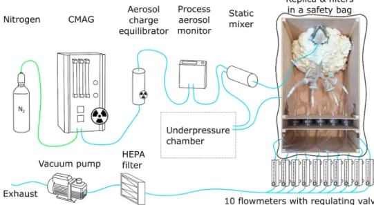
Aerosol particles were produced by Condensation Monodisperse Aerosol Generator (CMAG; model TSI 3475, TSI Inc. Shoreview, MN, USA), see Fig. 3. The particles were generated utilizing controlled heterogeneous condensation of DEHS vapour on small particles of sodium chloride. This process enabled the production of sufficiently high concentrations of monodispersed aerosol (up to 105 particle/cm3) with mean aerodynamic diameters3 of 2.5–3 μm continuously measured by a process aerosol monitor (model TSI 3375).
The aerosol material entered a static mixer where it mixed with air to provide the required flow rate and was delivered into the airway replica through the mouth, nose or combined way according to the test case. An LDA was used to measure the particle motion inside the airway model.
The model was terminated at the 7th bronchial generation level and equipped with ten collectors, followed by hoses and flow meters with regulation valves to adjust appropriate individual flow rates (see Table 1). The outlets were connected to a joint pipe with a regulation valve to provide the total flow rate representing steady breathing regimes (30 and 60 L/min). A vacuum pump was used to maintain the airflow as a downstream suction source, which emulated the in vivo breathing where the flow is controlled by pressure reduction in lower airways.
A 1-component LDA system (Dantec Dynamics A/S, Skovlunde, Denmark) was used for point-wise measurement of the velocity of individual particles flowing through the airway model. A light beam with a beam waist diameter of 0.82 mm and power of 60 mW was emitted from Argon Ion continuous wave laser ILT 5500A-00 (Ion Laser Technology, Salt Lake City, UT, US) and expanded to 2.5 mm in diameter to reduce the probe volume. Spectral line 514.5 nm of the CW laser beam was split, using transmitting optics 58N10, into two parallel beams 60 mm apart. The frequency of one of the beams was shifted by 40 MHz. An ellipsoidal probe volume was formed at the beam crossing using a transmitting lens with 240 mm focal length. The measuring volume dimensions were 0.25 ×0.25 ×0.3 mm. The first-order refracted light from particles was collected at a forward scattering angle of 80–100◦through a receiving lens with 310 mm focal length using a Dantec 57X10 receiving optics equipped with a photodetector (high voltage was set to 1100–1260 V). The ellipsoidal probe volume was reduced at the receiver side with a slit into an approximately cylindrical shape with a diameter of 0.25 mm and length of 0.12 mm. A Dantec BSA P80 signal processor compiled the measured velocity data with the velocity centre and span set to 1.94–7.29 and 3.84–11.67 m/s respectively, depending on the flow regime. The processor was set to SNR =0 dB, signal gain 20 dB and level validation ratio =4. Minimum and maximum record length was 32 and 256 respectively. The measurement and obtained Fig. 3.A scheme of the test rig for flow velocity measurement with LDA and the airway replica. LDA configuration, data acquisition and processing.
3 Particles sized up to 3 μm were found to be good air flow tracers as their Stokes number in our experiments was always <0.1. According to Tropea, Yarin, and Foss (2007) the Stk <0.1 provides flow tracing accuracy with errors below 1%.
F. Lizal et al.
data were maintained using BSA Flow Software v5.2.
The experiments were performed with 50 000 samples or 10 s measurement duration. The velocity measurement at all selected points in the lung cast cross-sections was three times repeated. In the computational simulations, the points were adjusted to fit those of the experiments to allow result comparisons. The LDA measured 1-component velocity of individual airborne aerosol particles flowing through the airway model. The mean axial velocity of the particle flow (i.e. the velocity component normal to the corresponding cross- section of a tube in the airway model) was calculated from the measurements.
The total error in the velocity value estimation of the LDA measurements is expressed as a sum of the bias error and the mea- surement uncertainty. The bias error stems from the effect of the optical path (it is attributed to the optical distortions caused by the irregular model walls) and it produces a certain degree of over- or under-estimation of the velocity magnitude at the measurement point. The comparison of LDA and CFD results is also burdened with the errors in flow character caused by differences between the geometry of the experimental and CFD airway geometry.4
The random error sources include variations and uncertainties in boundary conditions and external issues (the fluid flow rate, fluid physical properties, the flow tracking capability of tracer particles (see footnote 3) and the LDA related effects (the positioning error of the LDA measurement volume, the electronic and optical noise, and the finite size of the measurement volume). Other errors such as the discretisation error for A/D velocity conversion are negligible.
Individual errors affect the velocity and TI measurements differently; the bias error applies only in the case of mean velocity, while the electronic and optical noise increase solely the RMS velocity.
The experimental system was carefully checked and aligned to minimize the experimental error. The bias error was found to be, depending on the model curvature and wall thickness, ±5% of the measured velocity in areas with good optical access (typically in the middle of the cross-section), however, it rose to ±25% in the vicinity of the curved airway walls. Fortunately, the bias error is minimized during the calculation of TI, as it is a ratio of the fluctuating velocity over the averaged velocity in the same point. Hence, the same bias error applies to both numerator and denominator and cancels out. The random error (A type uncertainty estimate) for velocity and TI, obtained as the standard deviation of repeated measurements, is 0.06 m/s and 0.4% respectively in all the model sections and for both flow rates.
The measurement precision and uncertainties of LDA measurements in the transparent airway models are concisely summarised in Lizal et al. (2018). The effect of positioning error on the match of experimental and CFD mean velocity was discussed in our earlier paper (Elcner, Lizal, Jedelsky, Jicha, & Chovancova, 2016).
2.4. Experimental measurement of deposition
2.4.1. The airway replica for particle deposition measurements
Measurement of deposition of inhaled particles was performed by PET. Requirements of this method were different from those for the flow measurements. Namely, the optical transparency of the replica was not a priority, whereas solidity of the walls was needed because the replica had to be transported from the exposition chamber to the scanner. For this reason, the whole replica was produced by rapid prototyping on the printer J750 (Stratasys, Eden Prairie, MN, USA) which uses PolyJet technology. Accuracy of the printer was 0.2 mm and the layer thickness was 14 μm. A photopolymer VeroClear (Stratasys, Eden Prairie, MN, USA) was used as a building material. The face mask which leads the aerosol to the mouth and nose was produced from acrylonitrile butadiene styrene (ABS) on Fortus MC 450 (Stratasys, Eden Prairie, MN, USA). The inner geometry of the replica was identical with the replica used for flow measurements and the geometry used for simulations. The thickness of the wall of the replica was 2–4 mm.
As the replica must remain motionless during the exposition, transport and scanning, it was fixed in a wooden box with spray foam.
Ten outputs of the model were connected to filters by hoses. The filters were also built-in to the wooden box (see Fig. 4).
2.4.2. Setup of the particle deposition measurements
The experimental procedure has been described in detail in Lizal, Belka, Adam, Jedelsky, and Jicha (2015). A crucial point of the method is the selection of a proper positron emitter. There are several positron emitters which can be considered as suitable tracers of inhaled particles. Fluorine-18, with its half-life of 109 min, is the most used PET radionuclide in medical applications, thanks to its good transportability, acceptably low positron energy contributing to high spatial resolution and rather easy preparation in cyclotrons in the form of the 18F-fluoride anion. The most used fluorine-18 radiopharmaceutical is 18F-fluorodeoxyglucose (FDG). In its con- ventional application, FDG is used as a metabolic tracer that is primarily taken up by tissues with high energy demands, which is typical of many growing tumours. The patient is injected with the radiopharmaceutical and then scanned by a PET/CT or PET/MRI scanner. For lungs, the method is routinely used for non-small-cell lung cancer and pulmonary nodules in oncology, and for pulmonary Langerhans cell histiocytosis and sarcoidosis (Prabhakar et al., 2008; Szturz et al., 2012). Likewise, fluorine-18 can be easily applied to fit the demands of the experiment on the 3D printed replica of airways.
For the current experiment, it was important to generate non-evaporating and non-condensing particles, whose diameter could be user-controlled. It is a common practice in aerosol research to use the principle of heterogeneous condensation of DEHS on suitable nuclei to produce such particles. For this experiment, the CMAG (TSI 3475, TSI Inc., Shoreview, MN, USA), which works on the above- mentioned principle, was used. Normally, micron-sized liquid particles are formed first by spraying water-sodium chloride solution
4 For discussion of the influence of small changes in the airway geometry please see (Kelly et al. 2004a, 2004b).
Journal of Aerosol Science 150 (2020) 105649
from the nozzle in the atomizer vessel. Then, the liquid particles are dried out by diffusional dryer to produce sodium salt crystals in the size close to 100 nm. For the current experiment, the setup was modified to produce positron-emitting nuclei. The original CMAG atomizer was replaced by a shielded one. The emitter - fluoride-18 nuclide - was prepared by 10-min irradiation of 2 mL of H218O enriched water by an 18 MeV proton beam in the IBA Cyclone 18/9 cyclotron. The irradiated water was transferred to a shielded dispensation cell and the fluoride was captured on a resin-filled purification column. The activity was eluted by 200 μL of saline solution in 2 mL of injection water. 6 GBq of activity (at the reference time) was transferred to the modified atomizer vessel of the CMAG.
The CMAG was placed in a shielded chamber during the experiment (see Fig. 4). The generated aerosol went through the 85Kr based NEKR-10 charge equilibrator (Eckert & Ziegler Cesio, the Czech Rep.) to avoid electrostatic deposition of particles inside the airway replica. The size and concentration of particles were monitored on-line during the whole exposure part of the experiment by an aerosol monitor (PAM, TSI 3375, TSI Inc., Shoreview, MN, USA). Detailed measurement of the particle size distribution at the face mask inlet was performed by Aerodynamic particle sizer (APS, TSI 3321, TSI Inc., Shoreview, MN, USA) at the beginning of the exposition. A static mixer was placed upstream of the replica to mix the aerosol with air to achieve the desired inhalation flow rate. The aerosol then entered the face mask and the replica. Non-depositing particles were collected downstream of each of the ten output branches on filters. The flowrate through the replica and its output branches was controlled by flow meters with regulating valves. The distribution of flow rates among the output branches is recorded in Table 1. All the output hoses were merged into a single line downstream of the flow meters. An additional HEPA filter was placed before the vacuum pump to remove any possible remaining radioactive particles.
The vacuum pump output led to an exhaust. For safety reasons, the replica in its wooden box was placed in a plastic bag, which was kept in underpressure to prevent any possible leakage of the radioactive aerosol to the environment.
The inner surface of the replica was not covered by any coating. The coating is used in some cases for two reasons. The first is to prevent bouncing of solid particles. That is supposed to correspond with the real lung environment, where the particle remains deposited once it hits the wall. As in our case liquid particles were used, no rebound was expected. The second reason for application of the coating is to prevent surface wetting (accumulation of the liquid on the surface and trickling down in drops). The exposure time of the models was in our case 5–15 min, depending on the decreasing level of radioactivity in the atomizer; therefore, the amount of deposited matter was not sufficient to create liquid film or droplets on the wall and the coating was not needed.
The exposition was performed for two flow rates (30 and 60 L/min). All types of inhalation, MB, NB, and CB, were measured for 30 L/min. Only MB and NB were measured for 60 L/min. The measurements were performed in two phases (the phases were several months apart). At first, the regimes with 30 L/min and particles with CMAD of 2.8 μm were measured. Then, during the second stage, particles with CMAD of 2.0 μm were used. The second stage started with a single measurement of NB for 30 L/min (to verify the repeatability of the experimental setup) and then the 60 L/min flow rate regimes were set. The replica was in an upright position during the exposition, thus simulating the deposition for standing or sitting person.
Each replica was quickly transported to a PET/CT scanner Siemens mCT Flow Biograph 64 (Siemens AG, Munich, Germany) immediately after the exposure. CT and PET images were recorded and subsequently analyzed in Carimas 2.9 (Turku PET Centre, Turku, Finland). For a detailed description of the analysis please see Lizal et al. (2015). Shortly, the replica was divided into 22 segments (see Fig. 1). A separate volume of interest (VOI) was created for each segment. Radioactivity in Becquerels was evaluated in each VOI by the Carimas software. Also, the radioactivity of the downstream filters and hoses leading to them from the output branches was evaluated. It was assumed that the activity in each segment is proportional to the number of deposited particles. Hence, the deposition fraction (DF) in the specific segment was calculated as a ratio of the radioactivity in the segment divided by total
Fig. 4. A scheme of the test rig for the measurement of particle deposition.
F. Lizal et al.
radioactivity in the whole replica, hoses and filters. Accuracy of this method is limited by the uncertainty of the scanner itself, with its most important source being positron range. The essence of this error stems from the fact that the scanner detectors register the position of positron annihilation, not emission. Uncertainty is also brought in by the image analysis with subsequent evaluation of radioactivity (for details see (Lizal et al., 2015; Lizal et al., 2018)).
3. Results 3.1. Flow field
The results in this section were acquired from measurements in five cross-sections in the trachea (SA, SB, SC, SD and SE). The presented SA-SE lines lie in the sagittal plane (Fig. 5). The other three measuring lines lie immediately above the first bifurcation (CA), in the right main bronchus (CrB), and in the bronchus intermedius (CC), all of them in the coronal plane.
The fate of the inhaled particles depends on the airflow characteristics along the transport path. A systematic comparison between the nasal, oral and combined inhalation (indicated as NM, MB, CB in the figure labels) was provided under 30 and 60 L/min flow conditions for CFD simulations and LDA experiments in the same geometry to gain insight into the overall and local flow conditions in the respiratory tract. The description here does not focus primarily on the general explanation of the flow features, which are given in an extensive way elsewhere (Elcner et al., 2016; Zhang & Kleinstreuer, 2011), but rather to specific flow features that depend on the inhalation route.
The development of the mean axial5 velocity profile in five consequent positions in the central sagittal plane in the upper airways is resolved in Fig. 6. The corresponding flow profiles for 30 and 60 L/min are very similar to each other, which suggests similar flow structures in this flow range in agreement with Phuong and Ito (2015). Only minor structural variations appear: the velocity magnitude of 30 L/min profile (after a two-times multiplication to correct the flow rate difference) is ~4–14% larger in the central region (DN =
− 0.35 to 0.3)6, while the 60 L/min profiles are flatter in the near-wall regions. This is caused by the increased momentum exchange in the boundary layer that corresponds to the higher Re value of the 60 L/min regime.
The flow profile in the cross-section SA (oropharynx) is naturally significantly affected by the inhalation route. The nasal breathing (NB) features a sharp velocity peak near the posterior pharynx wall due to the jet produced by local flow constriction in the naso- pharynx. While the second half of the velocity profile (DN =0 to 0.5) shows negative velocity values and suggests for a recirculating flow present in the anterior oropharynx part. The mouth breathing (MB) produces a jet which spans through the anterior half of the cross-section and leads to increased velocity in that part compared to the posterior half. The combined breathing (CB) features a more uniform velocity profile. The nasal channel provides a higher flow resistance and it delivers only 8.7 and 13.1% (data taken from the CFD simulations) of the total air mass for 30 and 60 L/min respectively, but the nasal air portion comes with high momentum.
However, the CB profiles (also for other sections) always differ less from the MB than the NB profile as the mouth flow dominates. The flow profiles develop to a more uniform shape downstream of the glottis. The differences in the profiles due to the inhalation route are still evident in the cross-section SB (hypopharynx), namely in the shear layer positions (DN ~ (0.35, 0.45) and (− 0.35, − 0.45)) but gradually diminish for consequent cross-sections. The uneven and bent shape of the trachea causes alternate inclination of the flow to one or other side and presence of recirculation regions.7 It is reflected in the profiles that are somehow deflected (SC) or inclined to any of the sides (SD, SE).
The TI from LES and experimental data was calculated as a ratio of a square root of the variance (i.e. standard deviation, which is equal to RMS value) of axial velocity divided by a mean of axial velocity in the examined point. It is dimensionless. There are several ways of calculating TI. The RMS value can be divided either by a mean velocity averaged over the measuring cross-section or over the replica inlet, or divided by the local mean velocity value (in the measuring point). The latter method suits best for investigation of the regional features of the flow and hence was selected in this study.
The profiles of TI were plotted to reveal the level of velocity fluctuations which could retain the history of the flow, i.e. the imprint of the inhalation route might be noticeable in the TI profiles further downstream compared to the velocity profiles. The hypothesis that the flow disturbances formed in the upper airways may persist for several generations of bronchial airways downstream before becoming attenuated was formulated by Olson, Sudlow, Horsfield, and Filley (1973) and later presented by other authors, e.g. (Luo, Hinton, Liew, & Tan, 2004). Further support for this hypothesis can be found in Koullapis, Nicolaou et al. (2018). They have studied the flow in three different upper airway geometries. Fig. 9 demonstrates that three different mean velocity profiles at A1A2 lead to roughly the same profile at D1D2. However, three different turbulence profiles at A1A2 lead to different turbulence profiles at D1D2 (of course in the same geometry). It indicates that the reaction of mean velocity to the change of the geometry is faster than the reaction of fluctuations to the same change.
The current results have shown that although there were significant differences between the inhalation routes in the cross-section in the oropharynx (SA), and especially the NB regime generated very high fluctuations, the second cross-section immediately upstream of the vocal cords (SB) showed only small differences and all the remaining downstream profiles looked almost identical.
From the profiles SD and SE in Fig. 6 it might seem that the high TI correlates with low-velocity gradients. However, it is probably
5 It is the velocity component parallel to the normal vector of the inspected cross-section.
6 The normalised diameter, DN, in Figs. 6 and 7 represents the distance from the axis of the tube divided by its diameter.
7 For an overview of the flow in the extrathoracic airways and TB tree see Appendix A with the mean velocity magnitude and turbulence intensity contours.
Journal of Aerosol Science 150 (2020) 105649
just 13a rather specific feature of those two cross-sections. TI typically increases when the mean velocity drops down because the fluctuating velocity always features a non-zero value.
The flow profiles can be compared with results in Koullapis, Nicolaou, et al. (2018) where several computational approaches were employed on a model identical with our geometry except that it did not contain the nasal cavity. Our SA profile slightly differs from the reference, while the following profiles show a gradually better match in their shapes and values; the specific structures are well resolved and consistent. The relative differences between profiles calculated by LES by Koullapis et al. and the current CFD results (MB regime) were calculated in four cross-sections from the pharynx to the end of trachea (named C to F in the Koullapis’s paper). The relative differences in the consecutive cross-sections were 8.4, 8.1, 5.9, and 4.7%, respectively. The drop of values means that the profiles become closer to each other. The biggest difference in the upper profile is probably a consequence of the presence of the nasal cavity in our case, which influenced the flow profile although the MB regime with closed nostrils was used for comparison. The relative difference was calculated in the following way. The two curves of velocity profiles in the respective cross-sections were subtracted from each other. As a result of this operation, a curve showing relative differences between the two profiles was acquired. The relative difference was then calculated as a ratio of the absolute area under the curve divided by the area under the velocity profile curve of Koullapis (the figures with the comparison are presented in Appendix A, Figs. A10− A13).
3.1.1. Bronchial tree
Results in three coronal cross-sections, CA (Trachea), CrB (Right main bronchus) and CC (Bronchus intermedius) labelled according to Fig. 5 are documented in Fig. 7, for conciseness.8 The whole flow field is documented in Appendix A, Figs. A1− A8. The simulated profiles of mean axial velocity and TI are complemented with available experimental data from LDA measurements to document the match of the experimental and simulated results. The LDA was able to measure the flow velocity in multiple cross-sections of the transparent lung model cast; in each of these cross-sections, several points were measured, depending on optical access.
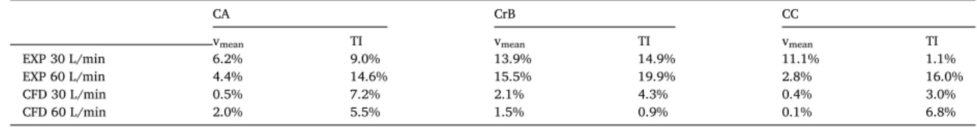
The simulated velocity profiles are very similar between the different inhalation routes. In the same way as in the extrathoracic flows, the CB profiles are closer to the MB than to NB profiles when evaluated in detail. The maximum relative local differences of the mean velocity in a point of the cross-section between NB and MB are 2.0–5.5% and 1.4–6.8% for 30 and 60 L/min respectively, as documented in Table 2. No systematic pattern was found for local differences either for the individual cross-sections or the flow rates.
At the same time, there is no qualitative difference among the profiles, indicating that the inhalation route does not induce any flow effects or alter flow structures in this airway part.
The corresponding velocity profiles for 30 and 60 L/min are very similar in shape; the velocity magnitude of 30 L/min profile is, after normalisation by the flow rate, by several percents larger in the central region while the 60 L/min profiles are flatter in the near- wall regions.
The velocity profile in the CA cross-section shows two indistinct lateral peaks due to a stagnation point at the carina (the internal ridge at the bifurcation of airways). The peak directed to the right lung is slightly higher due to high asymmetry in the flow distribution into the two lungs, with the left and right lung receiving 29 and 71% of the air respectively. (This significant flowrate asymmetry is Fig. 5.The scheme of measuring lines in the airway geometry, and visualization of the central sagittal plane and the coronal plane with an indication of the cross-section positions.
8 The cross-section was chosen with the aim of demonstrating the flow development in the complicated bifurcated system and to point out specific flow features in the consequent lung branches.
F. Lizal et al.
given by the constriction of the current geometry at the end of segment 4. The constriction comes from the original source - reference airway geometry according to Schmidt et al. (2004)). The CrB cross-section is placed in the detachment region of the right main bronchus and so the profile shows a decrease in velocity on the right side (DN ~ (− 0.45, − 0.25)) due to flow separation (see Appendix A, Figs. A1 and A5). There are also large velocity differences between the inhalation routes resulting in larger percentual differences compared to the CA profile placed upstream. The CC profile is flat with no specific features and very low route-induced velocity differences.
The main sources of differences between experimentally measured velocities and CFD in the CrB cross-section are the experimental uncertainties at that point. They stem from a highly irregular shape of the replica wall of the replica, which resulted in a combination of bias and positional error accumulated at that point. The error influences the magnitude of the measured velocity. However, since it influences fluctuations and the mean velocity in the same way, it cancels out when those two are put in a ratio to calculate TI (see Fig. 6.The mean axial velocity (left) and turbulence intensity (right) profiles in consequent positions of the central sagittal plane in the upper airways for nasal, oral and combined inhalation at 30 and 60 L/min flow rates. Negative values of the DN stand for anterior direction and positive for posterior.
Journal of Aerosol Science 150 (2020) 105649
Fig. 7.The mean axial velocity (left) and turbulence intensity (right) profiles in cross-sections of the trachea (CA), the right main bronchus (CrB) and bronchus intermedius (CC) of the coronal plane in the TB airways for nasal, oral and combined inhalation at 30 and 60 L/min flowrates.
Negative values of the DN stand for lateral direction and positive for medial.
Table 2
Maximum local differences between NB and MB in mean velocity within a profile related to average cross-sectional velocity.
cross-section \ flow rate 30 L/min 60 L/min
CA 3.7% 5.1%
CrB 5.5% 6.8%
CC 2.0% 1.4%
F. Lizal et al.
section 2.3 for details).
The simulated TI profiles in all three cross-sections do not show any significant difference between the 30 and 60 L/min flow rates.
The TI value spans between 0.05 and 0.15 for most of the cross-section (DN ~ (− 0.35, 0.35)) in each case. The only exception is the CrB position for DN around − 0.3, where TI increases up to 0.6–0.8 due to the presence of flow separation (see Appendix A, Figs. A3 and A7).
No systematic qualitative or quantitative differences between the inhalation routes are seen for TI both for simulated and experimental data.
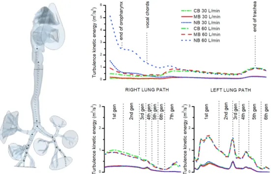
To precisely monitor the development of velocity fluctuations, the centreline turbulence kinetic energy (TKE) was plotted from the oropharynx (starting at the cross-section SA) down two paths – to the outputs with the largest flowrate in the right and left lung (segments 18 and 15, respectively; see Fig. 8). The results show that the initial disturbances induced in the nasal cavity dampen very fast and no difference can be observed downstream of the glottis. Surprisingly, bifurcations are not a common source of disturbance.
The highest levels of TKE are reached in the left main bronchus and then at the end of the second generation (segment no. 6). Smaller peaks can be found in the fourth generation of the left lung path and in the right main bronchus.
3.2. Results of experimentally measured and simulated deposition of particles
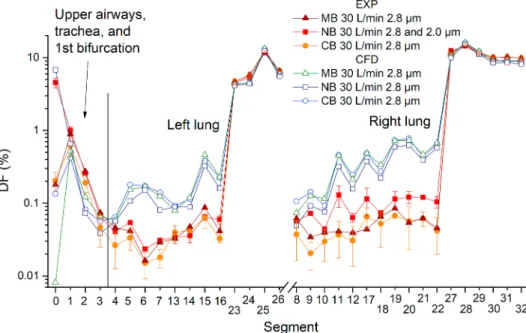
Deposition fraction shows the percentage distribution of inhaled particles. The results in the following charts contain both CFD and experimental results (Figs. 9 and 10). Experimental data acquired from the PET are depicted as an average of two measurements where the error bars show the difference between two repetitions of the same regime. No error bars are printed when only one experimental result was available. The filters placed downstream of the terminal segments were labelled with numbers 23–32 in Figs. 9 and 10.
When n is the number of a specific terminal segment, then its respective filter number is always n +10.
Obviously, most particles penetrated through the whole replica and deposited on the output filters, while the distribution of deposition among the filters was directly proportional to the flow rate through the respective filters. The vertical axes in the main graphs in Figs. 9 and 10 are on a logarithmic scale to facilitate observing of differences between the experiments and CFD, as this graphical presentation visually emphasizes smaller scales. To keep the general notion of a full picture, the graphs with linear scales are inserted in Appendix A, Fig. A14-A15.
Focusing first at the experimental and CFD results separately, the influence of the inhalation route can be observed. Experimental results indicate that the differences between inhalation regimes are low, especially for the first measurement phase with a flow rate of 30 L/min. The CB and MB provided almost identical results for 30 L/min; therefore only NB and MB was measured during the second experimental phase with inhalation of 60 L/min.
The distribution of deposited particles among replica segments remained unchanged regardless of the flowrate and inhalation route except, of course, the deposition in the oral and nasal cavities alone. It should be noted that the NB regime for 30 L/min was measured twice, but not within one day but once during each experimental phase, while slightly different particle sizes (2.8 vs. 2.0 μm CMAD) were used. Nonetheless, the results of the repeated measurements were remarkably similar.
It is important to mention that the initially established flow rates decreased slightly (from 30 to 25 L/min, and from 62 to 58 L/min)
Fig. 8.The course of turbulence kinetic energy (TKE) along the centreline passing from oropharynx through the airway with the largest diameter in the left and right lung down to 7th generation of branching for 30 and 60 L/min.
Journal of Aerosol Science 150 (2020) 105649
during the replicas exposition time due to the heating of the vacuum pump and due to increasing pressure resistance of the filters as particles deposited on them. It was not possible to adjust the flow rates during the course of exposition due to radiation prevention and safety reasons.
CFD results at a flow rate of 30 L/min confirmed that CB and MB produced almost identical deposition pattern. However, unlike experiments where the NB deposition was higher in many replica segments, it was consistently slightly lower in CFD than CB and MB.
Another notable difference between CFD and experiments was in the MB regime - while CFD predicted almost zero deposition in the nose, the experimentally obtained value was almost as high as for CB. In general, experiments showed higher deposition in the oral cavity and the trachea but lower deposition in all the remaining segments of the replica. Although the differences between CFD and experiments are low in terms of absolute values (the median of differences in DF between the respective segments as calculated by CFD and measured experimentally for the flow rate of 30 L/min was 0.26%), the consistency of the experimental and CFD results indicate Fig. 9.Comparison of deposition fraction (DF) measured experimentally and calculated by CFD for a flow rate of 30 L/min and all three inhala- tion routes.
Fig. 10.Comparison of deposition fraction (DF) measured experimentally and calculated by CFD for a flow rate of 60 L/min and all three inha- lation routes.
F. Lizal et al.