And Control of Nonlinear Process Systems
Ph.D. Thesis
Gábor Szederkényi
Supervisor: Professor Katalin Hangos
Information Science Ph.D. School
Department of Computer Science
University of Veszprém
Veszprém, Hungary
2002
Analysis And Control Of Nonlinear Process
Systems
Értekezés doktori (PhD) fokozat elnyerése érdekében
Írta:
Szederkényi Gábor
KészültaVeszprémi Egyetem InformatikaiTudományokDoktoriIskolájakeretében
Témavezet®: Dr. Hangos Katalin
Elfogadásra javaslom(igen / nem)
(aláírás)
A jelölta doktori szigorlaton ...%-otért el
Veszprém ...
aSzigorlatiBizottság elnöke
Az értekezést bírálókéntelfogadásrajavaslom:
Bíráló neve: ... (igen /nem)
(aláírás)
Bíráló neve: ... (igen /nem)
(aláírás)
A jelöltaz értekezés nyilvános vitáján ...%-ot ért el
Veszprém ...
a BírálóBizottság elnöke
A doktori (PhD)oklevélmin®sítése ...
...
AzEDT elnöke
Nemlineáris folyamatrendszerek diagnosztikája, analízise és irányítása
szürke doboz módszerek segítségével
A disszertációbanaszerz®speciálisdinamikusrendszerosztály, atermodinamika
törvényeialapjánm¶köd® folyamatrendszerek diagnosztikájával,analízisével ésirá-
nyításávalfoglalkozik. Vizsgálattárgyaazis,hogyanemlineárismódszerekalkalma-
zásávalkapotteredmények milyen zikai,termodinamikaijelentéssel rendelkeznek.
A szerz® értekezésében megmutatja, hogy a dinamikus folyamatmodell mellett
rendelkezésre álló szürke doboz hibamodellek alkalmazása kedvez®en befolyásolja
a vizsgált hibadetektáló és hibadiagnosztikaialgoritmusoktulajdonságait, és mód-
szert adahiba térbelilokalizációjáraa folyamatdinamikaimodellneka jelektérbeli
elhelyezkedését is gyelembe vev® nomítása útján. A felhasznált eszközöket és
az eredményeket a szerz® h®cserél® hálózatok modell-alapú hibadiagnosztikájának
példáján szemlélteti.
Az értekezés els® részében a szerz® a modellek állapot-irányíthatóságát és zéró
dinamikájátvizsgálja nemlineáristechnikákkal.
A nemlineáris állapot-irányíthatósági analízis elvégzése általános esetben nehéz
feladat, de aszerz® megmutatja, hogy bizonyos folyamatmodell-osztályok(félfolya-
matos üzem¶ bioreaktorok) speciális struktúrálistulajdonságainakfelhasználásával
a forrásfüggvény konkrét alakjától függetlenül analitikusankiszámítható az a nem-
lineáriskoordináta-transzformáció, amellyelfelismerhet®kazállapotváltozókbeme-
nett®l függetlennemlineáris kombinációi.
A szerz® a zéró dinamika analízisével bemutatja, hogy folyamatosüzem¶ biore-
aktoroknálhogyanválaszthatóolyankimenet,amelynek szabályozása révén a rend-
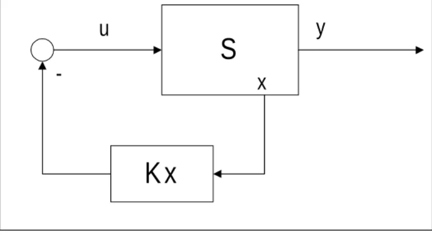
szer globálisan stabilizálható. A szerz® ezen kívül a lineáris optimális szabályozás
ésanemlineárisrendszerek közti kapcsolatfelhasználásávaláltalánosanhasználható
módszert ad arra, hogy nemlineáris input-an állapottér modelleknél hogyan vá-
lasztható ki legalább lokálisan aszimptotikusan stabil zéró dinamikával rendelkez®
lineáriskimenet.
A folyamatmodellek széles osztályát leíró dinamikus modellek ún. egyszer¶ ha-
miltonialakrahozhatók. A szerz®értekezésében megadja afolyamatrendszerek ha-
miltoni leírásánaka rendszer forrásfüggvényére vonatkozó feltételét, és a visszacsa-
tolt rendszer globális stabilitásvizsgálatánalapuló módszert ad a hamiltoni szabá-
lyozókhangolására.
Grey-Box Approach For The Diagnosis, Analysis And Control Of
Nonlinear Process Systems
The primary goal of this dissertation is to investigate how modern analysis tech-
niquesdeveloped fornonlinear input-anestatespacemodels canbeutilizedinthe
controland diagnosis of nonlinear process systems exploiting the special structural
propertiesof process models.
Usingtheexampleofmodel-basedfaultdiagnosisofheat-exchangers, itisshown
that the performance of the fault detection and isolationalgorithmsis improvingif
agrey-box modelof the investigated fault isused together with the process model.
It isshown ontheexample offermentationprocesses, thatthe generallycompu-
tationally complex problem of nonlinear reachability (controllability) analysis can
be analyticallysolved for special classes of process systems.
Using the notion of zero dynamics the author proposes methods toselect those
outputsofprocess modelswhichare appropriateforthe localorglobalstabilization
of the system.
Alargeclassofprocesssystems canberepresentedinthe so-calledsimplehamil-
tonianframework. Inthe thesis,amethodisgiven forthetuningofthehamiltonian
controllersand an important condition of the hamiltonianrepresentation is given.
Diagnostik, Analyse und Überwachung von nichtlinearischen
Prozess-Systemen mithilfe der Grau-Box-Methoden
Das Primärziel dieser Dissertation ist zu untersuchen, wie die für die nichtlinearen
Zustandsraummodelle in Input-An-Form entwickelten modernen Analysentech-
niken in der Überwachung und der Diagnostik der nichtlinearen Prozess-Systeme
unter Verwendung der speziellen strukturellen Eigenschaften der Prozessmodelle
anzuwenden sind.
Am Beispielder Fehlerdiagnostikder Wärmetauscher auf Modellbasiszeigt uns
derAutor, dass dieVerwendung desneben demdynamischenProzessmodellverfüg-
baren Grau-Box-Fehlermodells die Eigenschaften der geprüftenFehleraufdeckungs-
und Fehlerisolationsalgorithmengünstig beeinusst.
Der Dissertation ist es am Beispiel von Fermentationsprozessen zu entnehmen,
dassdienichtlineareErreichbarkeits-(Steuerbarkeits-)Analyse,dieimnormalenFall
einkomplexes Problembedeutet, beigewissen Modellklassenauchanalytischgelöst
werden kann.
Unter Verwendung desBegrisder Zerodynamikempehlt unsder AutorMeth-
oden zur Auswahl der Ausgaben der Prozessmodelle, die fürdielokaleoder globale
Stabilisierungdes Systems geeignet sind.
Eine breite Klasseder Prozess-Systeme istinder sog. einfachen Hamilton-Form
zu beschreiben. In der Dissertation gibt der Autor eine wichtige Bedingung der
einfachen Hamilton-Beschreibung bezüglich der Quellenfunktion an und gibt eine
Methode zur Einstellung der hamiltonischen Regler.
1 Introduction 14
1.1 Motivation and aim . . . 14
1.2 Contributions and layout of the thesis. . . 15
2 Model-Based Diagnosis of Heat Exchangers 17 2.1 Motivation . . . 17
2.2 Literature review . . . 18
2.2.1 Basicconcepts . . . 18
2.2.2 Approaches to faultdetection and diagnosis . . . 19
2.2.3 Important design issues. . . 19
2.2.4 Process and fault models . . . 20
2.2.5 System identicationand parameter estimation . . . 20
2.2.6 Detectingchangesin signals . . . 21
2.2.7 Evaluationof fault detection and diagnosismethods . . . 21
2.2.8 Models and methods- steps of the solution . . . 21
2.3 Process modeling . . . 22
2.3.1 The modelinggoal . . . 23
2.3.2 Modelhierarchies . . . 23
2.3.3 Modeling forfault detection . . . 24
2.4 Case study: the countercurrent heat exchanger . . . 24
2.4.1 Models on various levels of detail . . . 24
2.4.2 Fault modeling . . . 26
2.5 Measurement data ltering . . . 28
2.6 Parameter estimation . . . 30
2.6.1 Linear cascade model- allmeasurements available . . . 30
2.6.2 Linear cascade model- onlycold side measurements available 34 2.6.3 Oversimplied model . . . 39
2.6.4 Bilinearcascade model . . . 41
2.7 Fault detection and diagnosis . . . 41
2.7.1 Detectingjumps inthe heattransfer coecient . . . 41
2.7.2 Detectingdecrease inthe cold side liquidvolume . . . 42
2.7.3 Employing the change detectors simultaneously . . . 43
2.8 Tuning knobs of the algorithms . . . 44
2.9 Simulation results . . . 45
2.9.1 The simulatedheat exchanger . . . 45
2.9.2 Oversimplied model . . . 46
2.9.4 Bilinearcascade model . . . 47
2.10 Summary . . . 47
3 Nonlinear Model Analysis 51 3.1 Motivation and basic notions. . . 51
3.2 Reachability of input-anesystems . . . 52
3.2.1 Controllabilityof linear systems . . . 52
3.2.2 Reachability of nonlinear systems . . . 53
3.2.3 Algorithmfor generating the reachability distribution . . . 55
3.2.4 Example: linear systems . . . 56
3.3 Dissipativity and passivity . . . 57
3.4 The zero dynamics . . . 58
3.4.1 The zero dynamicsof SISO nonlinear systems . . . 58
3.5 Modeling, analysis and control of continuous and fed-batch fermen- tation processes: ashort literature review. . . 59
3.6 Reachability of continuous fermentation processes . . . 61
3.6.1 State space modelof the fermenter . . . 61
3.6.2 Controllabilityanalysis . . . 62
3.7 Reachability of fed-batch fermentation processes . . . 64
3.7.1 Problemstatement . . . 64
3.7.2 Nonlinearstate space model . . . 64
3.7.3 Reachability analysis . . . 65
3.7.4 Calculationof the coordinates transformation . . . 67
3.7.5 Generalizations . . . 70
3.7.6 Engineeringinterpretation . . . 73
3.7.7 Comments onobservability. . . 73
3.7.8 The minimalrealization of fed-batch fermentationprocesses . 74 3.8 The zero dynamicsof continuous fermentation processes . . . 75
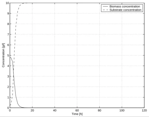
3.8.1 Selecting the substrate concentration as output . . . 76
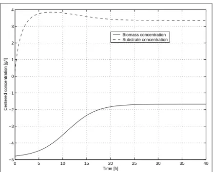
3.8.2 Selecting the biomass concentrationas output . . . 76
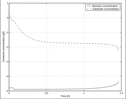
3.8.3 Selectingthe linearcombinationofthe biomassandsubstrate concentrationsas output . . . 77
3.9 Stability analysis of continuous fermentation processes . . . 77
3.10 Summary . . . 79
4 Analysis Based Control Structure Selection 81 4.1 Motivation . . . 81
4.2 Static controller design and performance analysis . . . 82
4.2.1 The controlproblemstatement and comparison viewpoints . . 82
4.2.2 Pole-placement controller. . . 83
4.2.3 LQcontrol. . . 84
4.2.4 Localasymptotic stabilizationvia feedback linearization . . . 85
4.2.5 Passivity based control . . . 89
4.2.6 Evaluationand comparison of the controllers . . . 91
4.3 Output selectionfor feedback linearization . . . 92
5 Hamiltonian View on Process Systems 95
5.1 Motivation . . . 95
5.2 Introduction . . . 95
5.3 Simple Hamiltoniansystem models . . . 96
5.4 Nonlinear State Equation of Process Systems . . . 98
5.4.1 Generalassumptions . . . 98
5.4.2 Normalizedsystem variables . . . 99
5.4.3 The transfer term inthe conservation balance equations . . . 99
5.4.4 Decomposition of the state equation driven by mechanisms . . 100
5.5 The simpleHamiltoniansystem modelof process systems . . . 101
5.5.1 Input variables for the Hamiltoniandescription . . . 101
5.5.2 The Hamiltonianfunction of process systems . . . 102
5.6 Passivation and loop-shaping based onthe Hamiltoniandescription . 104 5.7 Case study: anonlinear heat exchangercell . . . 106
5.7.1 Conservation balances and system variables . . . 106
5.7.2 Extensive-intensive relationships . . . 106
5.7.3 Normalizedsystem variables . . . 107
5.7.4 Decomposed state equationin inputane form . . . 107
5.7.5 Hamiltoniandescriptionof the heat exchanger cell. . . 108
5.8 A simpleunstable CSTRexample . . . 108
5.8.1 Conservation balanceequation and system variables . . . 109
5.8.2 Hamiltoniandescription . . . 109
5.8.3 Passivity analysis of the unstable CSTR . . . 110
5.8.4 Passivation and loop-shaping of the unstable CSTR: illustra- tion of the controller tuningmethod. . . 110
5.9 Summary . . . 111
6 Conclusions 115 6.1 Theses . . . 115
6.2 Publications . . . 117
6.2.1 Publicationsdirectly related tothis thesis . . . 117
6.2.2 Otherpublications . . . 119
6.3 Directions for future research . . . 120
6.4 Tézisek magyarnyelven . . . 120
A Detailed Simulation Results of Chapter 4 123 B Mathematical tools 131 B.1 Notations, basic tools and concepts . . . 131
B.1.1 State space representation . . . 131
B.1.2 Changes of coordinates (coordinates transformations) . . . 131
B.1.3 Lie-derivative . . . 132
B.1.4 Lie-product . . . 133
B.1.5 Distributions . . . 133
B.1.6 Codistributions . . . 134
B.3 Conservation matrices and their properties . . . 136
B.4 Quadratic forms and denitematrices. . . 137
B.5 Stability of nonlinear systems . . . 137
This thesis summarizes the contributions of my research work for obtaining Ph.D.
degreein Information Science at the IntelligentSystems Laboratory of the Depart-
mentof ComputerScience at the University of Veszprém. The scientic part ofthe
studies was mostly undertaken at the Systems and ControlLaboratory, Computer
and AutomationResearch Institute of the HungarianAcademy of Sciences.
This workwould never have been written withoutthe help, continuous support
and encouragement of several people. First of all, I want to express my sincere
gratitude tomy supervisor, Professor KatalinHangos, for her excellent andpatient
guidance throughout my studies.
I would also like to thank Professor József Bokor, the head of Systems and
ControlLaboratory for introducingmetorobust controland for providingmewith
the essential literature on nonlinear controlsystems. Next, let me thank Professor
ZsoltTuza, ProfessorFerenc Szigeti,Zoltán Szabó,ZsoltBíró, andGáborBacsófor
answering my mathematical questions. I would also like to thank Professor Tibor
Vámosfor thestimulatingdiscussionsand forhelpingmetosee importantconcepts
fromabird'seyeview. I'malsogratefultomyfellowstudents,PiroskaAiler,Mihály
Kovács, Balázs Kulcsár, Tamás Péni, Barna Pongrácz, Gábor Rödönyi, and István
Szászifor the jointwork. Furthermore,thanks toallthe people atthe Systemsand
Control Laboratory forthe helpful and supporting environment.
Finally, I'm grateful to my parents for supporting my studies in many ways for
sucha long time.
The partial support of the Hungarian National Science Foundation through
grantsNo. T017108, T026575 and the EU-Copernicusproject CT94-0237 is grate-
fully acknowledged.
Basic mathematical symbols
x2X x isan element ofset X
x2= X x isnot an element of set X
xY X isa subset of set Y
; empty set
[ union
N the set of natural numbers
R the set of real numbers
C the set of complex numbers
R n
n-dimensionalreal space, n2N
R +
the set of positivereal numbers
R +
0
the set of non-negative real numbers
I nn
n-dimensionalunit matrix
v T
transpose of the vector v
Notation for state space models
x state vector (x: AR !X R
n
)
u input vector (u: AR !U R
p
)
y=h(x) outputvector (y : AR !Y R m
)
_ x=
dx
dt
time derivativeof the state vector x.
@f
@x
Jacobi-matrixof the function f : R n
!R n
; x! f(x)
dh=
@h
@x
gradient vector of the functionh: R n
!R
reachability distribution
[f;] spanff;g
i g; g
i
2; i=1;:::;q
hh
1
;h
2
;:::;h
m
ji the smallest distributionwhich contains and
is invariantunder the vector elds fh
1
;h
2
;:::;h
m g.
?
annihillator of adistribution at apointx,
whichis the set of covectors that annihillateallvectors in(x)
?
(x)=fw
2(R n
)
:<w
;v >= 0for allv 2(x)g
tection
t
s
samplinginterval
Æ the delta-operator: Æy(k)=
y(k+1) y(k)
t
s
forgettingfactor of the RLSalgorithm
S
u
cumulative sum calculated fromthe discretetime signal u
threshold level for change detection
Y(s) Laplace-transformof the continuous time signal y: R +
0
!R at s2C
Notation of the variables and parameters of process
systems
heat exchangers
v ow rate
T temperature
V balance volume
U heat transfer coecient
A heat transfer area
c specic heat
density
bioreactors
X biomass concentration
S substrate concentration
F input feed owrate
S
F
substrate feedconcentration
Y yield coecient
reaction rate (source) function
max
;K
1
;K
2
kinetic parameters in
Notation for Hamiltonian systems
q generalized coordinates
p generalized momenta
H(p;q;u) Hamiltonianfunction
chemical potential
P thermodynamical driving force
V potentialenergy
CUSUM cumulative sum
FDLTI nite dimensional linear time-invariant
HTC heat transfer coecient
LQR linear quadratic regulator
LS least squares
LTI linear time-invariant
LTV linear time-varying
MIMO multiple-inputmultiple-output
RLS recursive least squares
SISO single-input single-output
w.r.t. with respect to
Introduction
Problems cannot be solved at the same
level of awarenessthat created them.
/Albert Einstein/
The analysis and control of nonlinear process systems is a rapidly developing and
important area of systems and control theory. This thesis presents new results
in this eld. Topics covered by the thesis are quite diverse in terms of the tools
and techniques used. Theseare parameter estimation, model-based faultdiagnosis,
nonlinear and Hamiltonian analysis and control of dynamic models. However, a
commonidea ispresent throughout the work: how the special structural properties
of process systems can be used to simplify these tasks. This approach is called
grey-box modeling.
1.1 Motivation and aim
The rst chapter of the thesis deals with model-based fault detection and isolation
of process systems. Dynamicprocess plantsare becomingmore and more complex,
therefore there is a growing demand for fault detection and diagnosis in order to
provide safe and continuous operation. Fault detection and diagnosis are playing
anincreasingly important role in the process industries, too. Dynamic modeling of
the equipments, called operating units is a well developed area, and model based
diagnostic methods can thereforebeeciently and relatively easilyapplied.
The usualdesigngoalofprocess systemsistocreateenergy and/orcost optimal
systemswhichisoftenahighlycomplicatedproblem. Mostoften, linearizedmodels
are used formodelanalysis and controllerdesign. However, the dynamic behaviour
of process systems is known to be nonlinear in most cases due to the complex
thermodynamic relations,reactionkinetics etc. On the other hand, more and more
theoreticallywell-groundedmathematicaltoolsforstudying nonlinearsystems have
become available recently. The naturalform ofa process modelisa nonlinear state
spacemodelwithclearengineeringmeaning. Therefore,theaimofthesecondpartof
theworkwastoapplythetoolsofnonlinearmodelanalysisandcontroltorelatively
simple but practicallyimportantprocess system classes.
the applied methods in his and my work do not overlap each other. In [96], [97],
[94], [98] and [95] the authors investigate the properties of process systems with
techniques developed for LTIand LTV systems.
1.2 Contributions and layout of the thesis
Thethesisconsistsof5chapters(notcontainingthisIntroduction)andanAppendix
of 2 parts. Each chapter begins with a motivation part that describes the main
problem statement and aimof the corresponding part. The motivation is followed
byabriefliteraturereviewofthemostimportantscienticresultsthatareneededfor
understanding the forthcomingsections. Thechaptersare nishedwitha summary
where the conclusions are drawn.
Thelayoutofthethesisandthemainscienticcontributionsaredescribedbelow.
Chapter 2 Model-baseddiagnosticmethodsfornonlinearprocesssystemsarestud-
ied in this part. I investigate how the increasing level of detail of process
modelsand the availabilityof measurementdata inuence the qualityof fault
detection and isolation algorithms. It is also shown how useful the available
priorinformationisabout the natureof the faultstobedetected. The results
are illustrated onthe exampleof countercurrent heat exchangers.
Sections 2.12.3 contain the basic notionsfrom the eld of model-based fault
detection and process modeling,while the main scientic contributions of the
thesis are insections 2.42.10.
Chapter 3 In this chapter, I apply nonlinear analysis methodsfor the state space
models of nonlinear process systems and compare the results with the tradi-
tional linear techniques. It is shown that nonlinear reachability analysis (if it
isanalyticallycomputable)givesmore informationabout the operationofthe
processthan linearanalysis. It isalsopresented that theconcept andanalysis
ofzerodynamicsisextremelyusefulforproperoutputselectionforbothlinear
and nonlinear controller design. The examples that illustratethe aboveideas
are continuous and fed-batch fermentationprocesses.
The general description of the investigated system properties together with
a literature review on modeling, analysis and control of simple bioreactors
are containedinsections 3.13.5,and the main contributions are described in
sections3.63.10.
Chapter 4 In this part, the results of Chapter 3 are used for the controller de-
sign of continuous fermentation processes. Several types of static linear and
nonlinear controllers are designed and compared here. The results of Chap-
ter 3 help to understand the (sometimes unexpected) behaviourof the closed
loopsystems. At the end of this chapter, a generallyapplicable linear output
selectionmethod for nonlinear controlis described.
The motivation for this chapter is contained in section 4.1, and the main
contributions are insections 4.24.4.
nonlinearprocess systems. Themainresultsofthispartistheconditionunder
which a non purely convective process system can bedescribed in the simple
Hamiltonianframework and the tuning of Hamiltoniancontrollers.
The motivation for the chapter and a brief introduction into the theory of
Hamiltonian systems are contained in sections 5.15.3, and the main contri-
butionsare described in sections5.45.9.
Chapter 6 This chapter contains the nal conclusions of the thesis and describes
the possible directions of future research.
Appendix A Thispart of the Appendix contains simulationresults for Chapter 4
that couldn't be tto the main text due tospace limitations.
Appendix B This part summarizes the necessary mathematical denitions and
theorems used in the thesis fromthe area of nonlinear controlsystems.
Model-Based Diagnosis of Heat
Exchangers
2.1 Motivation
Theaimofthechapteristoshowhowprocessmodelingaectstheresultofthefault
diagnosisandisolation. Forthispurposedierentprocessmodelsofthesamesystem
are investigated whichdescribe the process system onvarious levelsof details. The
faultdetection properties, namely the sensitivity, detection delay and selectivity of
thefaultdetectionmethodappliedfordetectingthesamefaultareshowntodepend
onthe levelof detail of the process model.
The concepts and methodsare illustrated onasimple but practicallyimportant
case study, on the example of detecting heat exchange surface deterioration and
leakage faults in countercurrent heat exchangers. The simulation and evaluation is
performed using the model-based fault detection toolbox developed in a COPER-
NICUS project [88].
Heatexchangers are widelyused inthe processindustries andother areas. They
are usually arranged in units containing several (5-200) of them. From a modeling
point of view, heat exchangers are among the simplest and most investigated oper-
ating units for which we have both reliabledynamic models with known properties
and accumulated operationalexperience. This experience can be used in formulat-
ingsuitabledynamic models of the typical faultswhichcan beencountered inheat
exchangers.
Model-basedfaultdetectionmethodsare proposedinthischapter. Themethods
are based on a rst principle model of the operating unit: a countercurrent heat
exchanger, and on the grey- and white box models of the faults: the deterioration
ofthethe heattransferbyagingand theleakingofthe outercontainer. Wepropose
to use recursive parameter estimation methods with a forgetting factor to track
the heat transfer coecients (HTCs) and the liquid volume in the outer container
respectively. Thesettled materialbreakage faultisdetected via detectionof abrupt
positive jumps in the estimated heat transfer coecient using a detector based on
a cumulative sum (CUSUM) test. The leakage fault is detected by estimating the
liquidvolumein the outer container and then applyingthe CUSUMtest again.
The possibility to detectfaults in any industrialequipment heavily depends on
tothe in- and outows of the equipment (ow rates and temperatures) are usually
measured but measurements along the equipment are rarely available. Therefore
the possibilities of fault location in space are rather limited. The proposed fault
detection methods have variants corresponding to various modeling assumptions:
the oversimplied model, the linear cascade modeland the bilinearcascade model.
It is stressed that the investigations in this chapter were made under idealistic
assumptions(perfectmodelingofthefault-freeprocess,Gaussian-typemeasurement
noise).
2.2 Literature review
Thepurposeofthis sectionistobriey discussthebasicconcepts offaultdetection,
diagnosis and compensation and to review the most important scientic results in
this eld that are closely connected to the topic of this chapter. It is also a task
here to place the models and methods used in this chapter among the dierent
approaches that are surveyed.
2.2.1 Basic concepts
Fault detection is the indication that something is going wrong in the system via
various residual generation methods. A residual is such a function of time that is
nominallyzero orclose tozero whenno faultispresent, and thatis distinguishably
dierent from zero when a certain component of the system fails [54]. The task of
faultdiagnosis istodeterminethetype,sourceandextentof thefaultaswellasthe
time of its occurrence based on the observed analytical and heuristic knowledge of
the symptoms. In otherwords, faultdetectionand diagnosisisthe earlyindication
of incipient faults that can help us toavoid major plant breakdowns and catastro-
phes and take appropriate actions in order to maintain the operation. The main
task of fault compensationis to modify the normal mode conguration in order to
compensate for the faults(if possible)by activating various back-upsystems [104].
We can say that the detection and compensation of faults is one of the critical
issues in the operation of high-performance systems: production equipment such
as power stations, chemical processes, transportation vehicles like airplanes, space
vehiclesetc.
Fault detection,diagnosisandcompensationschemesinplantsdetectand tryto
compensate faults in one or more of the following three subsystems: the actuator,
the process (or plant) and sensor subsystems. Actuator faults are discrepancies
between the intended controland itsrealization by the actuators. Sensor faultsare
discrepancies between the measured and true values of the plant's output or input
variables. Process faults are disturbances actingon the plant causinga shift inthe
plantoutputs independently of the measured inputs, and may describe plantleaks,
overloads,brokendown componentsetc. Withrespecttothe dierentsectorswhere
the faults may occur, one can distinguish between actuator fault detection, sensor
faultdetection and process faultdetection.
Approaches to fault detection and diagnosis are divided into three main streams:
model-free methods, model-based methodsand knowledge-based methods.
Model-free methods do not make use of a plant model. Limit value checking,
whichisoneofthem,mostoftenworkswelliftheprocessoperatesapproximatelyin
asteadystate. Thebigadvantageofthesemethodsistheirsimplicityandreliability.
But their application becomes more involved if the process changes frequently and
rapidly itsoperating point. Sincethe plant variables may vary widely due to input
variations, the setting of the check threshold is often a nontrivial task. Further
problems may arise from the installationof special sensors and repeated hardware
elements that are usually distributed spatially around the system to provide pro-
tection against localized damage. The major causes of the problems in this case
are the extra cost and software requirement and the additional space needed to
accommodate the equipment.
Model-based methods rely on the idea of analytical redundancy based upon
theoretical ideas, signal analysis and process analysis. Signal analysis is performed
throughdirectlymeasurablesignalsbyusingsignalmodelslikecorrelationfunctions,
frequency spectra, autoregressive moving average, statistical decision theory etc.
Also, these methods use process analysis by using mathematical process and fault
modelstogetherwithparityspace,stateestimation,parameterestimation,detection
ltering,variable threshold logic etc. [33].
Knowledge-based redundancy complements the analyticalmodel-based method.
In addition to the symptom generation with model-based method, heuristic symp-
tomscanbeproducedby usingqualitativeknowledgeprovided byhumanoperators.
Such a method usually consists of a combination of logical rules, where each con-
clusion can, in turn, serve as a symptom in the next rule until the nal conclusion
is reached.
2.2.3 Important design issues of fault detection systems
Thedesignoffaultdetectionsystems demandsthethoroughconsiderationofseveral
issues and tradeos. Based on [104] the most important properties are as follows.
Rapid response isausualrequirementsincethe quickdetectionof faultsisofcrucial
importanceinmost cases. Noisesensitivity giveshowsensitivethedetectionsystem
is to certain high frequency eects. It is easy to notice that there is a tradeo
between rapid response and noise sensitivity. Increased noise sensitivity usually
results in a greater number of false alarms (fault is detected in spite of the fact
thatthe processoperatesnormally). Anotheritem thatisalsoofteninconictwith
rapid response is the degradation of system performance using a given detection
method. The robustness of a fault detection scheme in the presence of modeling
errors is also of major importance in most practical cases. In addition to these
issues the designer of fault detection systems should consider further questions in
connectionwithsoftware. Theseare computationalcomplexity,storagerequirements
and time requirements. Finally, it is an essential consideration, how the system
takes advantage of new computer capabilities and structures (e.g. designs that can
be implemented ina modularor parallelway).
Since the procedures that are going to be discussed in further sections are based
on mathematical process and fault models, a short classication and description
of such models is presented here. Generally speaking, a model is a tool for de-
scribing and understanding the world, it is a formal expression of our knowledge
corresponding to the investigated phenomena [75]. Dierent classes of models are
forexamplefunctional,physicalandmathematicalmodels. Inmathematicalmodels
the relations between the variables of the system to be modelled are mapped into
certainmathematical structures such asalgebraic-, dierential-,integral equations,
logical functions etc. The knowledge represented by a mathematical model can be
classied intothe followingfourcathegories: laws, structure, parameters and states
[75]. Laws are fundamental physical laws that determine the formof the equations
in mathematical models. Structure refers to the inner structure of the phenomena
andtotherelationsbetweenitsparts. The parametersofamathematicalmodelare
the particular values of the coecients standing in the equations. A state is such
a variable that describes the process of the investigated phenomena together with
outsideeects actingon the system.
According to the a priori information we have concerning the process, models
can be classiedintothe followingthree groups. Ifwe donot haveany information
about the structure and the parameters of the process, we use black box models.
All we are able to do in this case is to make inferences based on the knowledge of
the inputs and outputs of the system. When we have partial knowledge about the
structure (and maybe about some parameters) of the system we speak about grey
box models. Here we have a better understanding of the system than in the case
of a black box model, but it stillremains an incomplete view. When we know the
complete structure of the system and some (or even all) of itsparameters, we have
a white box model. Here our knowledge of the system and its internal workings is
virtuallycomplete, though someparts or subsystems may remaingrey boxes.
2.2.5 System identication and system parameterestimation
System identication gives solutions to two main problems: model parameter esti-
mationand modelstructure estimation [24].
Theproblemstatementofmodelparameterestimationisasfollows. Wearegiven
a measurement record (input and output values), acertain model form (structure)
and a loss function measuring the dierence between the measured and estimated
data. The goal is to estimate the model parameters from the data available that
minimizethe lossfunction. Theproblemstatement ofmodelstructure estimationis
the following. We are given ameasurement record (input and outputvalues),a set
of candidate models (modelstructures) and alossfunction. The aimin this case is
toselect the optimal structure that minimizesthe loss function.
Theapproachtosystemidentication,mostofthenotationsandthebasicmeth-
ods for parameter estimation are from [51] and [48]. Both books have served as
essentially important literature in this eld for more than a decade. Furthermore,
an excellent tutorial survey of parameter estimation algorithms for time varying
systems is [50].
The eld of fault detection and diagnosis is closely connected to detecting changes
incertaincharacteristicsignals[104]. Thesechangescanbeabruptorslowandthey
may refertothe presence of dierentkinds of faultsinthe system. Thus, detecting
these changes reliably and quickly plays an essential role in making the binary
decisionwhether the system isinfaultyornormal operationmode. The core ofthe
change detection algorithms used in this work were taken from [6] which became
a fundamental reference for engineers and researchers involved in fault detection,
diagnosisand many other elds inrecent years.
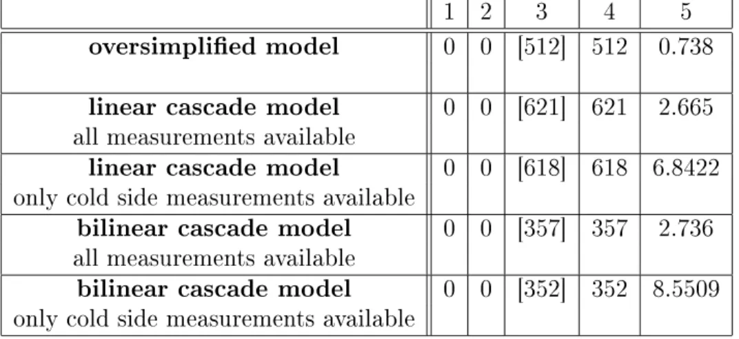
2.2.7 Evaluation of fault detection and diagnosis methods
Forthe purpose of evaluationof the fault detection and isolationmethods we need
measurablecharacteristicfeaturesofthemethodsaccordingtowhichthecomparison
of the solutions becomes possible. In the case of only a single fault and a fault
detectionmethodthe followingstand-alonefault detectionpropertiesareused based
onthe features oered by the Matlab Fault Detection Toolbox [106].
1. Fault detection false alarms (FDfalsealarms)isthenumberofdiscretetime
points in which the method detected the presence of some fault but no fault
occurred in reality.
2. Fault detection missed alarms (FD missed alarms) is the number of time
instants inwhichthe methoddidn'tdetect any faults,but some fault(that is
detectable by the method)occurred inreality.
3. Detection delays (DDs) is avector containingthe time delays(the number of
samplinginstants)passed between the actualoccurrence and the detection of
the faults.
4. Mean of detection delays (Mean of DDs) is the mean of the numbers inthe
Detection delays vector.
5. Mops is the number of million oating point operations required by a given
method asit ismeasured by Matlab's FLOPSfunction [105].
2.2.8 Models and methods - steps of the solution
Withthe summaryof the models andmethodsused inthis work,the outline ofthe
solutionsteps is alsosummarized here.
As ithas been mentioned intheMotivation ofthis chapter, the objective ofthis
work is to develop fault detection and diagnosis methods for countercurrent heat
exchangers. The aim is to detect two types of faults: the deteriorationof the heat
transfer surface (i.e. howCaCO
3
settleson and leavesthe surface) and the leaking
ofthe outercontainer. From this itis clearthat both faultstobedetected occur in
the process (or plant) subsystem.
ing heat exchangers are available from the literature and engineering practice, the
application of model-based methodsto solve the task isa reasonable choice.
The designissues ofthe taskcan be examinednowonthebasis of Section2.2.3.
Of course,rapid response and low noisesensitivity are importantgoals inthis case.
The tradeo between them can be handled quite successfully by using the known
properties of the process and setting the appropriate tuning knobs of the meth-
ods. Since the process that takes place in heat exchangers is rather slowcompared
to certain rapidly changing mechanical or electrical systems, the implementation
of the developed fault detection methods to microprocessor-based digital systems
practicallydoesnotcause any degradationinsystemperformance. Because of their
simpleimplementation, rapidness,smallcomputationalcomplexityand lowstorage
requirements,the application of recursive identicationalgorithmswas chosen.
In order to complete our task we need mathematical models that describe the
operation of the heat exchanger and the two faultsto be detected. The continuous
time heat exchanger model is a white box model that is in the form of ordinary
dierentialequations. Inthis model,we know the physicalmeaningof each param-
eter. The faultmodelof leakage isalso a white box model. The fault modelof the
settling CaCO
3
is based on prior heuristic knowledge of the phenomena where we
know which parameter carries the diagnostic information, therefore this is a grey
box model.
Fromthemodelsweknowwhichparametersaretobeestimatedinordertodetect
thefaults,meaningthatweencounter amodelparameterestimationproblematthis
step, which is solved by employing various recursive algorithms.
Afterdesigning the identicationmethods, the next stepistochoose and design
the procedures that detect changes in the estimated parameters. The actual fault
detection and diagnosis decisions are made on the basis of the results of change
detection.
The followingstep isthe implementationand, nally,the evaluationofthe fault
detection methods according tothe properties listed inSection 2.2.7.
It is widely known that one of the key steps in developing a powerful fault
detectionandisolationmethodisthestepofmodeling(seee.g.[34])Whenbuildinga
model,themodelinggoal,inourcasefaultdetectionandisolationplaysanimportant
role determiningthe type and precision of the required model[23].
2.3 Process modeling
Process modeling aims at constructing a mathematical model of a process system
suitablefor a given purpose. Therefore the problem statement of process modeling
requires tospecify the
process system together with the processes or controlling mechanisms deter-
miningits behaviour, and the
modeling goal determiningthe required modeltype and accuracy.
anisms, such as detailed reaction kinetics with all of the kinetic parameters, are
known exactly for the modeler. In this case, the methodology of grey box model-
ing is applied. However, the modeling focus should be put to the important model
elements fromthe viewpoint of the modeling goal.
2.3.1 The modeling goal
Themodelinggoalisfaultdetectionand isolationinthischapter. Thisimpliesthat
adynamicprocess modelis needed describing thefault-free process dynamicsto be
able todetectthe fault. Moreover, amodelorseveral models are requiredtomodel
the fault orfaultsto be isolated.
There is no need to achieve uniformly high precision of the predicted output
behaviour but rather the modelingfocus should be put on the distinctive elements
of the model for fault detection and isolation. In other words, both the fault-free
dynamic model and the fault model(s) should describe the processes and details
important forfault isolationpurposes.
2.3.2 Model hierarchies
Modelsofthesameprocesssystemforthesamemodelinggoalarerelatedandcanbe
arranged to various modeling hierarchies. There are levels in a modeling hierarchy
driven by some model property. One may arrange models of a process system
startingfromasimplestlinearinput-outputmodelwithrstorderdynamicsthrough
the most detailed nonlinear model which includes all the controlling mechanisms.
This is a hierarchy driven by the level of detail. Note that because of the fault
detectionandisolationgoalthe faultmodelshouldalsobepartoftheprocessmodel
driven by the level of detail.
The following levels driven by the level of detail are usually distinguished for
faultdetection and isolation purposes.
1. Top level: Lumped linear dynamics ("Oversimplied model")
Here the simplestrst order lumped linearinput-outputmodelof the process
system and that of the fault(s) is considered.
2. Middle level: Distributed or higher order linear dynamics ("Linear cascade
model")
Higher order linear lumped input-outputmodelis used in the middle level in
order to capture either the detailed approximate dynamics of a distributed
parameter process system or that of a higher order system and the faults
considered.
3. Bottom level: Distributed nonlinear dynamics ("Nonlinear model")
The most detailed nonlinear higher order lumped parameter input-output
models are used here in order to incorporate all the known and important
details.
The dynamic model is seen as a lter which is used to estimate the fault sensitive
ingredient(s)ofthe measureddata. In otherwordstheeect ofthe knownfault-free
dynamics is ltered out from the data using the process model. The fault model
part isused forfault detection and isolationpurposes thereafter.
2.4 Case study: the countercurrent heat exchanger
Theconcepts andresultsare illustratedonthe exampleofsurface deteriorationand
leaking ina countercurrent heat exchanger using models of various levels of detail.
2.4.1 Models on various levels of detail
Oversimplied model
On the top levelthe dynamics ismodeledbya singlepair of perfectlystirred lumps
forming a so called heat exchanger cell. Each cell consists of two perfectly stirred
tanks with in- and outows. The two tanks are connected by a heat transfer area
between them.
Themodelequationsforasinglecellconsistofthetotalmassandenergybalances
for the hot and cold sides respectively. In order to connect the top level model to
theotheronesthecellindexj (j =1)isusedforthesinglecell. Constantmass (and
thusconstantvolumeV
jh
with constantdensities
jc ,
jh
)isassumed inthehotside
thereforethe totalmass balanceispresent onlyforthe cold side. The equationsare
asfollows:
dT
jc
dt
= v
c
V
jc (T
(j+1)c T
jc )+
U
j A
j
c
pc
c V
jc (T
jh T
jc
) (2.1)
dT
jh
dt
= v
h
V
jh (T
(j 1)h T
jh )+
U
j A
j
c
ph
h V
jh (T
jc T
jh
) (2.2)
dV
jc
dt
= v
jl
(2.3)
T
(j+1)c
=T
ci
; T
jc
=T
co
; T
(j 1)h
=T
hi
; T
jh
=T
ho
(2.4)
where the subscripts h and c denote the hot and cold sides respectively. T
hi , T
ci
and T
ho , T
co
are the inlet and outlet temperatures, v
h
and v
c
are owrates, v
jl is
the leaking owrate, V
jc
and V
jh
are the volumes,A the heat transfer surface area,
c
pc
and c
ph
the specic heats,
c
and
h
the densities and U
j
is the heat transfer
coecient (abbreviated as HTC). Note that all of the variables and parameters
above are positive by denition.
With only a single cell in g. 2.1.a. describing the heat exchanger the outlet
temperatures T
ho and T
co
of the heat exchangerare the same asthat of the cell. In
this case only two state variables fT
co
;T
ho
g are considered with a single triplet of
equations(2.1)-(2.3).
In case of the simplest top level model all the model parameters including the
owrates v
h
and v
c
are constants and the inlet temperatures T
hi
and T
ci
are the
input ordisturbance variablesonly.
T ci
T h o T hi
T c o T 3 c T 2 c
T n c
T 1 h T 2 h
T (n-1)h
...
...
n 2 1
T h o T hi T c o T ci
a b
v c
v h
v c
v h
Figure 2.1: a. Single heat exchanger cell; b. Cascade model of a countercurrent
heat exchanger
Linear cascade model
Thecountercurrentheatexchangerismodeledasasequence ofcascadedcellsabove.
Athreecellmodelisused(seeing. 2.1.b)asamiddlelevelcascade modelbecause
it can describe the dynamics of the heat exchanger well enough for fault diagnosis
purposes for majority of the industrialequipments.
With the three-cell model three set of modelequations (2.1)-(2.3)are usedwith
the followingvariablerelationsinstead of Eqs. (2.4):
j =1;2;3; T
4c
=T
ci
; T
1c
=T
co
; T
0h
=T
hi
; T
3h
=T
ho
(2.5)
The modelabovecan beregarded asalumped version ofthe distributedparam-
eter model of the heat exchanger, therefore the cells are associated with particular
spatiallocationsalongtheequipmentlength. Thestatevariablesoftheabovemodel
arethe temperatures ofthe coldand hot sidesand the coldside volumeinthe cells,
i.e.fT
1h
;T
1c
;V
1c
;T
2h
;T
2c
;V
2c
;T
3h
;T
3c
;V
3c
g. Ifanequidistantinspacelumpingisper-
formed, i.e. the parameters A
j
and V
jh
are the same for allcells then heat transfer
coecients U
1
;U
2
;U
3
carry spatialinformation.
Here again, allthe modelparameters includingthe owrates v
h and v
c
are con-
stantsand the inlettemperatures T
hi and T
ci
are the inputordisturbance variables
only.
Bilinear cascade model (Nonlinear model)
The nonlinearity of process models is caused either by the convective ow when
the owrate is alsoa dynamic variable (bilineartype nonlinearity) or by the chem-
ical reactions and other mechanisms appearing in the source term of the balance
equations. In our case only the bilinear type nonlinearity appears caused by the
convective ow.
Inthebottomlevelthree-cellbilinearcascademodelthreesetofmodelequations
(2.1)-(2.3)canbeusedwiththe variablerelationsEqs. (2.5). Butnowthe owrates
v
h andv
c
are time varying variablesand areinput ordisturbancevariablestogether
with the inlet temperatures T
hi
and T
ci .
There are two types of faults considered: the deterioration of the heat exchanger
surfaceand leakingintheoutercontainer. Empiricalgrey-boxmodelisusedforthe
deteriorationand physical white-box modelis set up for the leakage.
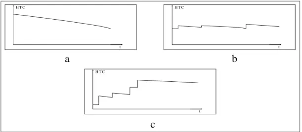
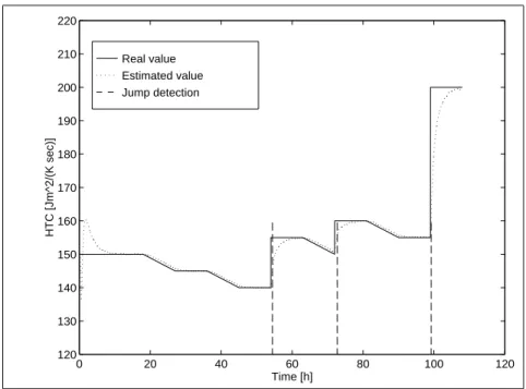
Deterioration of the heat transfer area
Under normal operating conditions the HTC is constant or slowly decreasing due
toalayerof settledmaterialbuildingup on theheat transfer surface (see g.2.2.a).
In oldheat exchangers large pieces of the settled materialcan break away fromthe
surface, causing damage in the equipment. When the settled material breaks o,
the HTCs will undergo abrupt positive jumps. These jumps can be grouped into
two qualitativelydierent types.
1. Inthe beginningwhenthe jumpsstart tooccur,they aresmall andinfrequent
becauseof the smallpiecesof CaCO
3
that leave theheat transfer surface(see
g.2.2.b).
2. Then in the later stages the jumps become large and frequent when bigger
'stones'of CaCO
3
comeo (see g.2.2.c).
The usual industrial practice is to wash heat exchangers with some kind of acid
between certain time intervals. However, this washing procedure requires the heat
exchangerandpossibly otheroperatingunitstobestoppedand thusitmay become
a rather expensive operation. On the other hand, if some information is available
abouttheprocessofthechangingoftheHTC,thenweareabletoavoidunnecessary
stoppings and damage caused by the settled material coming o the heat transfer
surface, too. Thus, one of the main ideas in this work is to track the HTC in the
heat exchanger and detect abruptpositivejumps in it.
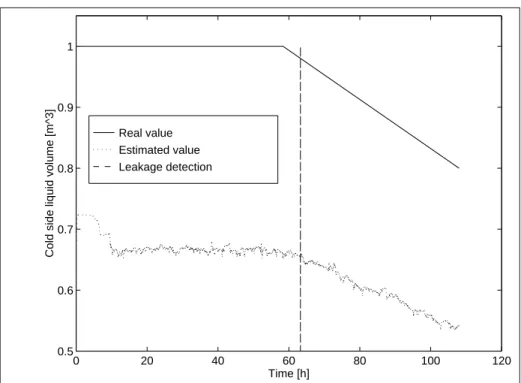
Leakage
When the outer container is leaking, there is an unmeasurable outow v
cl
on the
cold side from the heat exchanger (see Eq.2.3 and g.2.3) which may result in a
slowdecrease of the mass inthe outerphase, or- if the levelsare controlled, inthe
decrease of the outow from the equipment. Here it is assumed that the volume
ow rates v
h and v
c
are known and constant or measured, leaking can therefore be
detected via detection of a slow decrease in the cold side volume V
c
. Note that we
want to detect smallchanges in the cold side volume compared tothe initialvalue
ofthe volumeinthe heatexchanger. Thisisareasonableaimbecausethedetection
oflargeandquick changes(i.e. bigleaks)can beasimplertaskwithothermethods.
Moreover, there is no possibility to get spatial informationabout the leakage even
with our cascade model, since the liquid level on the cold side decreases uniformly
inthe whole heat exchanger. Thatis why itis importanttodevelop such a leakage
detectionalgorithmthatrequiresasfewtemperaturemeasurementdataaspossible.
H T C
t
H T C
t
H T C
t
a b
c
Figure 2.2: Three consecutive stages of the change of the heat transfer coecient:
a.Constant or slowly decreasing HTC; b.Smaller and infrequent jumps; c.Large
and frequent jumps
T hi T h o
T ci T c o
v h v h
v c v c
v cl T c o
Figure2.3: Leakage modelledas anunmeasurable outowfrom the cold side
Filteringis needed toavoidnumericaldierentiationof the noisytemperaturemea-
surements, because the forthcoming parameter estimation methodsrequire the ap-
proximationof the rst and secondderivatives of certainmeasured signals.
Numerical dierentiation is sensitive to noise and round-o errors (particularly
whenthesamplingintervalisshort),andlargeerrorsinthedierentiationcanoccur,
whichmayleadtonon-robustidenticationmethods. Thatis,themethodsmayfail
or have a very slow convergence in the presence of noise. The question is how can
we avoidtaking derivatives.
For adiscrete time signaly(k) the so-called Æ operatoris dened as[55]
Æy(k)=
y(k+1) y(k)
t
s
(2.6)
where t
s
is the samplingtime.
Assume we have an nth order discrete time system in the delta-operator (ob-
tained fromacontinuous time system), i.e.
A(Æ)y(k)=B(Æ)u(k) (2.7)
where the highest order occurring in the A and B polynomials is n. This means
thatthe nthorderderivativeofthesignalsisinvolved. Oneobviouswayof avoiding
taking this derivative is to integrate both sides of the equation n times, that is we
lter the signals through the lter 1
Æ n
. The system equation(2.7) then reads
1
Æ n
A(Æ)y(k)= 1
Æ n
B(Æ)u(k) (2.8)
and we see that 1
Æ n
A(Æ) and 1
Æ n
B(Æ) are now polynomials in 1
Æ
, i.e. we are now
integratingthesignalsinsteadoftakingderivatives. Thelter 1
Æ n
isjustoneexample
of a possible lter, but we have to integrate at least n times in order to avoid the
derivatives which means that the lter must be at least of order n (see [55]). This
means that if a particular parameter estimation algorithmrequires the rst or the
second derivative of certain signals then a rst or second order lter is applied on
the measurement data respectively.
The ideaofthe InniteImpulseResponse (IIR) lterdesigninour case isthata
continuous time lter is designed rst using the continuous time model of the heat
exchanger andthen the obtained lter istransformed into discretetime usingthe Æ
operator.
The generalmethodforconstructingsucha lterisasfollows[55]. Assumethat
acontinuous time system isgiven by the following input-outputmodel
Y(s)
U(s)
= B(s)
A(s)
(2.9)
the orderof B(s)). Thenthe lter thatshould beused is 1
A(s)
. After applyingthis
lter onthe system weget
Y(s)= B(s)
A(s)
U(s) (2.10)
To obtainthe discretetime lter, we substitute s in(2.10) for the Æ operator.
On the basis of the guidelines above, the lters that will be used in the fault
detection methods are the following.
First order lter. In this case we want to use a rst order lter with cuto
frequency !
c
=e
0
. The transfer function describing sucha lter is given by
F f
(s)
F(s)
= e
0
s+e
0
(2.11)
whereF(s)and F f
(s)are theLaplacetransformsofthe signaltobelteredandthe
lteredsignalitselfrespectively. The discretetimeversionof thislter iswrittenas
f f
(k)
f(k)
= e
0
Æ+e
0
(2.12)
fromwhichweget
Æf f
(k)= e
0 f
f
(k)+e
0
f(k) (2.13)
Tocalculatetheappropriateltercoecientinthiscase,letusselectfromEqs.(2.1)
and(2.2)theonethatdeterminesthedominanttimeconstantofoneheatexchanger
cell. Let us assume that this equation is Eq.(2.1), and that the cold side liquid
volume and the HTC in the heat exchanger are constant (i.e. we assume normal
operation). Let uswrite the Laplace transformof Eq.(2.1) inthe followingform.
T
jc
(s)(s+ v
c
V
jc +
U
j A
j
c
pc
c V
jc )=
v
c
V
jc T
(j+1)c (s)+
U
j A
j
c
pc
c V
jc T
jh
(s);j =1;:::;n (2.14)
According to the previously discussed lter design method, the rst order lter
coecient isas follows.
e
0
= v
c
V
jc +
U
j A
j
c
pc
c V
jc
(2.15)
where V
jc
and U
j
denote the nominal values of the cold side liquidvolume and the
HTC in the jth cellof the heat exchanger respectively.
Second order lter. Again we start from the transfer function of a continuous
time second orderlinear lter whichreads
F f
(s)
F(s)
=
e
0
s 2
+e
1 s+e
0
(2.16)
Converting it intodiscrete time gives
f f
(k)
f(k)
=
e
0
Æ 2
+e
1 Æ+e
0
(2.17)
Æ 2
f f
(k)+e
1 Æ
2
f f
(k)+e
0 f
f
(k)=e
0
f(k): (2.18)
Thecalculationof thesecondorderlter'sparametersfromthe heatexchanger's
parameters willbe shown inSection 2.6.2.
2.6 Parameter estimation
2.6.1 Linear cascade model - all measurements available
In this ideal and not too realistic case we assume that we have access to both the
hot andcold side temperatures ineachcellof the heatexchangerinadditiontothe
inlet temperatures. In other words, we know the temperature distribution along
the heat exchanger on both the cold and the hot sides. Furthermore, itis assumed
that A, c
pc , c
ph ,
c ,
h , V
h ,v
c
and v
h
are known. It must be admitted that it is
not often possible to measure the cold and especially the hot side temperature on
several points alongthe heat exchanger. On the other hand,we have agoodreason
toexpect thatweobtainthe mosteasilyimplementablealgorithmsinthis casethat
produce the most reliableestimates forthe parameters.
Estimating the HTC
An additionalassumption inthis case is that the cold side volume is constant and
known in the heat exchanger since the purpose of the algorithm discussed here is
onlyto give anestimate forthe HTC.
Using the gradient method with a forgetting factor 0 < < 1, it is possible to
obtain estimates directly for both U
jc
and U
jh
using the discrete time modelof the
heat exchanger. The forgetting factor means that old measurements are weighted
at an exponentially decreasing rate. (see [51]). Usingthe ltered temperatures we
can easilywrite the discretetime modelof the jth cellin the heat exchanger.
ÆT f
jc (k)=
v
c
V
jc (T
f
(j+1)c
(k) T f
jc (k))+
U
j (k)A
j
c
pc
c V
jc (T
f
jh
(k) T f
jc
(k)) (2.19)
ÆT f
jh (k)=
v
h
V
jh (T
f
(j 1)h
(k) T f
jh (k))+
U
j (k)A
j
c
ph
h V
jh (T
f
jc
(k) T f
jh
(k)) (2.20)
j =1;2;:::;n
One can see from(2.19)and (2.20) thatthe only unknown parameter inthis model
is the HTC, i.e. U
j
that carries the diagnostic informationabout the deterioration
of the heat transfer surface in the jth cell.
The prediction errors for (2.19) and (2.20)in the jth cellare given by
jc
(k)=ÆT f
jc (k)
v
c
V
jc (T
f
(j+1)c
(k) T f
jc (k)
U
j (k)A
j
c
pc
c V
jc (T
f
jh
(k) T f
jc
(k)) (2.21)
jh
(k)=ÆT f
jh (k)
v
h
V
jh (T
f
(j 1)h
(k) T f
jh (k)
U
j (k)A
j
c
ph
h V
jh (T
f
jc
(k) T f
jh
(k))(2.22)
j
U
j
(k) has tobecalculated
jc (k)=
@
jc (k)
@U
j (k)
= A
j
c
pc
c V
jc (T
f
jh
(k) T f
jc
(k)) (2.23)
jh (k)=
@
jh (k)
@U
j (k)
= A
j
c
ph
h V
jh (T
f
jc
(k) T f
jh
(k) (2.24)
Since we don't know the real value of U
j
we can approximate
jc
and
jh
in the
following way (see [51]).
^
jc
(k)=ÆT f
jc (k)
v
c
V
jc (T
f
(j+1)c
(k) T f
jc (k)
^
U
jc
(k 1)A
j
c
pc
c V
jc (T
f
jh
(k) T f
jc
(k)) (2.25)
^
jh
(k)=ÆT f
jh (k)
v
h
V
jh (T
f
(j 1)h
(k) T f
jh (k)
^
U
jh
(k 1)A
j
c
ph
h V
jh (T
f
jc
(k) T f
jh
(k)) (2.26)
The standardrecursivescheme for estimatingU
j
fromthe cold and hot siderespec-
tively is asfollows
^
U
jc (k)=
^
U
jc
(k 1)+p
jc (k)
jc (k) ^
jc
(k) (2.27)
p
jc (k)=
p
jc
(k 1)
jc +
2
jc (k)p
jc
(k 1)
(2.28)
^
U
jh (k)=
^
U
jh
(k 1)+p
jh (k)
jh (k) ^
jh
(k) (2.29)
p
jh (k)=
p
jh
(k 1)
jh +
2
jh (k)p
jh
(k 1)
(2.30)
Thechoiceof in(2.28)and (2.30) isatradeo between goodtracking capabilities
of the HTCs and sensitivity tonoise and unmodeled dynamics. A small value of
meansthat the estimatewilltrack variations inthe HTC quicker, but onthe other
hand,the itwillalsobecomemoresensitivetonoiseand unmodeleddynamics. The
actual estimates of the HTCs in the jth cell can be computed by using a convex
combination:
^
U
j
(k)=
^
U
jc
(k)+(1 )
^
U
jh
(k); 01 (2.31)
where shouldreect the relative condence wehave inthe two estimates.
Estimating the cold side volume
Theonlydierencebetweentheassumptionsinthisandthepreviouscaseisthatnow
theHTC ineachcellisassumed tobeknownand constantandthecold sidevolume
becomes a time-varying parameter. In most cases this is a reasonable assumption,
sincethechangeoftheHTCisusuallymuchslowerthanthatofthecoldsidevolume
during leakage. According to these assumptions the discrete time form of the cold
side energy balanceequation of the jth cellis given by
ÆT f
jc (k)=
v
c
V
jc (k)
(T f
(j+1)c
(k) T f
jc (k))+
U
j A
j
c
pc
c V
jc (k)
(T f
jh
(k) T f
jc
(k)) (2.32)
of the same size
V
jc (k)=
V
c (k)
n
(2.33)
where V
c
(k) denotes the overall cold side uid volume inthe heat exchanger and n
isthe number of cells the heat exchanger is divided into.
For the purpose of tracking the cold side uid volume let us introduce the fol-
lowing variable
V
jcr (k)=
1
V
jc (k)
(2.34)
Thuswe can rewrite (2.32)as
ÆT f
jc
(k)=V
jcr (k)v
c (T
f
(j+1)c
(k) T f
jc (k))+
U
j A
j V
jcr (k)
c
pc
c (T
f
jh
(k) T f
jc
(k)) (2.35)
Starting from (2.35) let us now present a possible identication scheme for the
trackingof the cold side uid volume.
Tracking with the gradient algorithm. Using (2.35) the prediction error is
writtenas
j
(k)=ÆT f
jc
(k) V
jcr (k)v
c (k)(T
f
(j+1)c
(k) T f
jc (k))
U
j A
j V
jcr (k)
c
pc
c (T
f
jh
(k) T f
jc
(k)) (2.36)
Its negative gradient with respect toV
jcr
(k) is given by
j
(k)=v
c (k)(T
f
(j+1)c
(k) T f
jc (k))+
U
j A
j
c
pc
c (T
f
jh
(k) T f
jc
(k)) (2.37)
The approximation of
j
(k) is writtenas
^
j
(k)=ÆT f
jc
(k) V
jcr
(k 1)v
c (k)(T
f
(j+1)c
(k) T f
jc (k))
U
j A
j V
jcr
(k 1)
c
pc
c
(T f
jh
(k) T f
jc
(k)) (2.38)
Using(2.38)and (2.37)therecursiveschemeforthe estimationofthe coldsideuid
volumecan bewritten as
^
V
jcr (k)=
^
V
jcr
(k 1)+p
j (k)
j (k)
j
(k) (2.39)
^
V
jc (k)=
1
^
V
jcr (k)
(2.40)
p
j (k)=
p
j
(k 1)
j +
2
j (k)p
j
(k 1)
(2.41)
where
j
is again a tradeo between quick tracking capabilities of the parameter
and sensitivity tonoise.
In this case both the HTC and the cold side volume are unknown parameters and
wewould liketoestimatethem simultaneously. An obviousstrategyto achievethis
goal is to combine the two algorithms described in Eqns.(2.23)-(2.31) and (2.37)-
(2.41) respectively. Within the jth heat exchanger cell we have two parameters
to be estimated in this case, namely V
jc
and U
j
. The idea of the solution is to
let the two gradient algorithms use each other's estimations. This approach works
very well if both V
jc
and U
j
vary slowly in time, but when abrupt jumps occur in
the HTC, problems arise with the estimation of the cold side liquidvolume. These
problems can be handled successfullyif weutilize allthe informationwehave from
the complete availabilityof measurement data.
The suitable form of the discrete time energy balance equation of the cold side
inthis case iswritten as
ÆT f
jc (k)=
v
c
V
jc (k)
(T f
(j+1)c
(k) T f
jc (k))+
U
j (k)A
j
c
pc
c V
jc (k)
(T f
jh
(k) T f
jc
(k)) (2.42)
while Eqn.(2.20) describing the hot side can be used here without change. After
combining the algorithms described in Eqns.(2.23)-(2.31) and (2.37)-(2.41) we get
thefollowingprocedureforthesimultaneousestimationofthecoldsideuidvolume
and the HTC inthe jthcell
jUcc (k)=
A
j
c
pc
c
^
V
jc
(k 1) (T
f
jh
(k) T f
jc
(k)) (2.43)
jUch (k)=
A
j
c
ph
h V
jh (T
f
jc
(k) T f
jh
(k)) (2.44)
^
jUcc
(k)=ÆT f
jc (k)
v
c
^
V
jc
(k 1) (T
f
(j+1)c
(k) T f
jc (k))
^
U
jc
(k 1)A
j
c
pc
c
^
V
jc
(k 1)
(2.45)
^
jUch
(k)=ÆT f
jh (k)
v
h (k)
V
jh (T
f
(j 1)h
(k) T f
jh (k))
^
U
jh
(k 1)A
j
c
pc
c V
jh
(2.46)
^
U
jc (k)=
^
U
jc
(k 1)+p
jUcc (k)
jUcc (k) ^
jUcc
(k) (2.47)
p
jUcc (k)=
p
jUcc
(k 1)
jUcc +
2
jUcc (k)p
jUcc
(k 1)
(2.48)
^
U
jh (k)=
^
U
jh
(k 1)+p
jUch (k)
jUch (k) ^
jUch
(k) (2.49)
p
jUch (k)=
p
jUch
(k 1)
jUch +
2
jUch (k)p
jUch
(k 1)
(2.50)
^
U
j
(k)= U
jc
(k)+(1 )U
jh
(k);2[0;1] (2.51)
jVc
(k)=v
c (T
f
(j+1)c
(k) T f
jc (k))+
^
U
j
(k 1)A
j
c
pc
c (T
f
jh
(k) T f
jc
(k)) (2.52)
^
jVc
(k)=ÆT f
jc (k)
^
V
jcr
(k 1)v
c (T
f
(j+1)c
(k) T f
jc (k))
^
U
j
(k 1)A
j
^
V
jcr
(k 1)
c
pc
c
(T f
jh
(k) T f
jc
(k)) (2.53)