Nemnegatív polinomiális rendszerek analízise és irányítása

(1)

Analysis and control of nonnegative polynomial systems

György Lipták

A thesis submitted for the degree of Doctor of Philosophy

University of Pannonia

Doctoral School of Information Science

Advisors:

Prof. Katalin M. Hangos Prof. Gábor Szederkényi

Veszprém, Hungary 2018

DOI:10.18136/PE.2018.671

(2)

Analysis and control of nonnegative polynomial systems

Értekezés doktori (PhD) fokozat elnyerése érdekében Írta: Lipták György

Készült a Pannon Egyetem Informatikai Tudományok Doktori Iskolája keretében.

Témavezető: Prof. Hangos Katalin Elfogadásra javaslom (igen / nem)

(aláírás) Témavezető: Prof. Szederkényi Gábor

Elfogadásra javaslom (igen / nem)

(aláírás) A jelölt a doktori szigorlaton ...%-ot ért el

Veszprém, ...

A Szigorlati Bizottság elnöke Az értekezést bírálóként elfogadásra javaslom:

Bíráló neve: ... (igen / nem)

(aláírás) Bíráló neve: ... (igen / nem)

(aláírás) A jelölt az értekezés nyilvános vitáján ...%-ot ért el

Veszprém, ...

A Bíráló Bizottság elnöke

A doktori (PhD) oklevél minősítése ...

...

Az EDT elnöke

(3)

Acknowledgements

First of all, I would like to thank my advisors Prof. Katalin M. Hangos and Prof. Gábor Szederkényi for their continuous support, guidance and encouragement during my studies.

I would also like to thank Prof. József Bokor and Dr. Bálint Vanek for the part time job in the Systems and Control Laboratory, Computer and Automation Research Institute.

I am also grateful for all the help I received from every member of the Systems and Con- trol Laboratory and the Department of Electrical Engineering and Information Systems, University of Pannonia.

I wish to express my gratitude to all my coauthors, Prof. József Bokor, Prof. Katalin M. Hangos,Dr. Tamás Luspay, Dr. Attila Magyar,Dr. Tamás Péni, Prof. Mihály Pituk, Dr. János Rudan,Dr. Zoltán Szabó, Prof. Gábor Szederkényi,Dr. Béla Takarics and Dr.

Bálint Vanek for their cooperation.

Last but not least, I am very grateful to my mother and father and to my whole family who always supported me in all possible ways.

Part of the work has been supported by the grants NF104706, K83440, K115694 and K120186 of the Hungarian Research Fund.

(4)

Abstract

The analysis and feedback control of nonlinear systems have been continuously developing in recent decades, because of their practical importance and challenging theoretical nature.

Kinetic systems are able to produce all the important qualitative phenomena present in nonlinear systems, so they form a dynamically rich-enough sub-class. It is well-known that the utilization of the physical and/or structural specialities of different nonlinear system classes greatly helps in obtaining theoretically well-grounded, powerful and practically still feasible analysis and control methods.

The realization theory of kinetic systems makes a connection between the structural properties and dynamical behaviour (e.g. complex balancedness, weak reversibility and deficiency). This makes it possible to develop efficient methods for their dynamical analysis.

The greatest difficulty of the realization based system analysis is that a system model may have more than one realization.

In this thesis, an optimization-based approach is presented for the computation of kinetic realizations with zero deficiency. The problem is traced back to the solution of an appropri- ately constructed mixed integer linear programming problem. Furthermore, it is shown that weakly reversible deficiency zero realizations can be determined in polynomial time using standard linear programming.

Feedback design methods are also proposed in this thesis for nonnegative polynomial systems with linear input structure. These methods are based on the optimization based realization computation methods, because the key dynamical properties of the closed loop can be easily prescribed with optimization constraints. The proposed methods are extended to nonnegative polynomial systems with parametric uncertainty, too.

Finally, a class of delayed kinetic systems derived from mass action type reaction network models is introduced. The time delayed positive stoichiometric compatibility classes and the notion of complex balanced time delayed kinetic systems are defined. The semistability of the equilibrium solutions for complex balanced systems with arbitrary time delays is proved.

(5)

Zusammenfassung

Die Analyse und Feedback-Kontrolle der nichtlinearen Systeme hat sich in den letzten Jahr- zehnten kontinuierlich aufgrund ihrer praktischen Bedeutung und der theoretischen Forde- rungen entwickelt. Die kinetische Systeme bilden eine breite, aber gut charakterisierbare Klasse der nichtlinearen Systeme und sie sind fähig, die wichtigste nichtlinierare Ereignisse zu beschreiben. Es ist aber auch bekannt, dass physische und/oder strukturelle Eigenschaf- ten verschiedener nichtlinearen Systemklassen sind verwendbar zur Analyse des Systems und der Planung der Rückkoplung.

Die Realisationstheorie kinetischer Systeme stellt einen Zusammenhang zwischen den strukturellen Eigenschaften und dem dynamischen Verhalten her (z. B. komplex-ausgeglichene, schwache Reversibilität und Defizienz). Die Realisationstheorie ermöglicht eine dynamische Analyse durch effizienten Methoden. Die größte Schwierigkeit der realisierungsbasierten Sy- stemanalyse besteht darin, dass ein Systemmodell über mehr als eine Realisierung verfügen kann.

In dieser Arbeit wird ein optimierungsbasierter Ansatz zur Berechnung von kinetischen Realisierungen mit Defizienz Null vorgestellt. Das Problem wird auf die Lösung eines entspre- chend konstruierten gemischten ganzzahligen linearen Programmierproblems zurückgeführt.

Weiterhin wird gezeigt, dass schwach reversible Defizienz-Null-Realisierungen in polynomiel- ler Zeit unter Verwendung von linearer Standardprogrammierung bestimmt werden können.

In dieser Arbeit werden auch Rückkopplung-Design-Methoden für nichtnegative Poly- nomsysteme mit linearer Eingangsstruktur vorgeschlagen. Diese Methoden basieren auf den optimierungsbasierten Realisierungsberechnungsmethoden, da die dynamischen Schlüsselei- genschaften der geschlossenen Schleife leicht mit Optimierungsbeschränkungen verordnet werden können. Die vorgeschlagenen Methoden werden auch auf nichtnegative Polynomsy- steme mit parametrischer Unsicherheit erweitert.

Abschließend wird eine Klasse von retardierten kinetischen Systemen vorgestellt, die von Reaktionsnetzmodellen des Massenaktionstyps abgeleitet sind. Die retardierten positi- ven stöchiometrischen Verträglichkeitsklassen und die Vorstellung von komplex-ausgeglichen retardierten kinetischen Systemen sind definiert. Die Semistabilität der Gleichgewichtslösun- gen für komplex-ausgeglichen Systeme mit beliebigen Zeitverzögerungen wurde nachgewie- sen.

(6)

Összefoglalás

A nemlineáris rendszerek analízise és irányítása az elmúlt évtizedekben folyamatosan fej- lődött, köszönhetően gyakorlati hasznosságának és az elméleti kihívásoknak. A kinetikai rendszerek a nemlineáris rendszerek egy tág, de jól karakterizált struktúrájú osztályát al- kotják, és képesek a legfontosabb nemlineáris jelenségek leírására. Ugyanakkor jól ismert, hogy egy-egy rendszerosztály fizikai és/vagy strukturális tulajdonságai jól alkalmazhatóak a rendszer analízisére és irányítás tervezésére.

A kinetikus rendszerek realizáció alapú analízise kapcsolatot teremt a strukturális és a dinamikus tulajdonságok közt, ilyen speciális tulajdonságok a komplex egyensúly, gyen- gén reverzibilitás és a deficiencia. A realizáció alapú analízis lehetőséget teremt a rendszer dinamikus analízisére hatékony módszereken keresztül. A módszerek nehézsége, hogy egy rendszer modell több realizációval is rendelkezhet.

A dolgozatban optimalizáción alapuló kinetikus realizáció keresési módszerek kerülnek bemutatásra. Az első módszer a nullás deficienciájú realizáció keresés problémáját oldja meg kevert egészértékű lineáris programozás segítségével. A második módszer a gyengén reverzibilis nullás deficienciájú realizációk számítására alkalmas. Ez a probléma lineáris programozás segítségével került megfogalmazásra, ami polinom időben megoldható.

Továbbá a dolgozatban állapot visszacsatolás tervezési módszereket adunk lineáris be- menettel rendelkező nemnegatív polinomiális rendszerekhez. A visszacsatolás tervezése op- timalizációs keretbe illeszthető, így a zárt rendszer legfontosabb dinamikus tulajdonságai könnyen előírható optimalizációs feltételek segítségével. A bemutatott módszer kiterjesztés- re kerül parametrikusan bizonytalan rendszerekre is.

Végül bevezetésre kerül az időbeli késleltetéssel rendelkező kinetikus rendszerek osztálya.

A pozitív sztöchiometrikus kompatibilitási osztályok és a komplex egyensúly tulajdonság kiterjesztésre kerül időbeli késleltetett esetre. A komplex egyensúlyi ponttal rendelkező kinetikus rendszereknek szemistabilitása bizonyításra kerül az időben késleltetett esetre.

(7)

Introduction

The analysis and feedback control of nonlinear systems have been continuously developing in recent decades, because of their practical importance and challenging theoretical nature [38]. Within the class of smooth nonlinear systems, polynomial systems form a well-studied class that enable us to apply computationally efficient methods for their dynamic analysis and control [74], and at the same time, have practically important applications in the field of process, mechanical, or (bio)chemical etc. control. Within this class, nonnegative polynomial systems play an important role in the applications, where the value of the variables is nonnegative by nature (e.g. concentrations, pressures, number of items in a set etc.). It is important to note that any bounded operation domain of a general non-positive system can be easily shifted into the nonnegative orthant.

1.1 Background and motivation

Because of the challenges in dynamic analysis and control of nonlinear systems and the significance of kinetic systems as a special class allowing the development of efficient methods, the work reported in this thesis is built upon results from a range of interdisciplinary areas including systems and control theory, optimization and differential equations briefly outlined in the following paragraphs. These areas form the background of the results achieved.

Polynomial kinetic systems The class of kinetic systems was proved to be a useful representation of smooth nonnegative system models not only in biochemistry, but also in other areas like population or disease dynamics, process systems, and even transportation networks [24, 33, 57]. A network-based description is often advantageous to describe key properties of potentially large, complex systems with many components [56, 45]. Kinetic systems are naturally equipped with a network (i.e. directed graph) structure called the reaction graph, which is the abstraction of a set of chemical reactions, where the chemical complexes and reactions can be represented by vertices and directed edges, respectively.

The detailed balance property of a thermodynamic system, defined originally by Boltzmann

(10)

in the 19th century, means that at equilibrium, each elementary reaction step is equilibri- ated by the corresponding reverse reaction. A more general condition is complex balance, which requires that the signed sum of incoming and outgoing reaction rates at equilibrium is zero for each complex in a kinetic system [36, 28, 23]. It is worth remarking that complex balance does not depend on a particular equilibrium (if there exist multiple equilibria in a system), but it is a property of a chemical reaction network itself [37]. For a historical re- view of the notions of detailed and complex balance, see [31]. Generally, complex balance is related to both the structure and the parameters of kinetic systems. First, complex balance implies that each component of the reaction graph is strongly connected (i.e. the reaction network is weakly reversible) [37]. It is also important that deficiency zero weakly reversible reaction networks are complex balanced for any positive values of the reaction rate coefficients [27, 26]. However, complex balance becomes a parameter-dependent property when the deficiency of the network is higher than zero.

The main significance of complex balance in systems and control theory stands in its stability implications [51]. According to the Global Attractor Conjecture, complex balanced kinetic systems are globally stable in the positive orthant with a logarithmic Lyapunov function that does not depend on the model parameters. The conjecture was proved for several special cases such as one linkage class networks [14], and a possible proof for the general problem has recently appeared in [20].

In (bio)chemical applications, the system parameters (typically the reaction rate coefficients) are uncertain, and often only their order of magnitude is known. Therefore, one of the main aims of the theory of kinetic systems is to give conditions on the qualitative behaviour of kinetic models using mainly the stoichiometry and graph structure of reaction networks [37, 27]. In [27] and [26], the authors introduce the study of the dynamics of kinetic systems as a function of a parameter known as the deficiency, which is a nonnegative integer not depending on the rate coefficients. A classical result of kinetic systems with clear significance in nonlinear systems theory is the Deficiency Zero Theorem that estab- lishes a robust stability property for deficiency zero reaction networks consisting of strongly connected reaction graph components [51].

It has been known for a long time, however, that the reaction network representation of a kinetic dynamics is generally not unique, i.e. reaction networks with different structures and/or different sets of chemical complexes may represent the same dynamics. This phe- nomenon is called macro-equivalence [37], confoundability [22] or dynamical equivalence [53], where the possible kinetic systems corresponding to the same dynamics are called realizations of a kinetic ODE model. The notion of linear conjugacy extends dynamical equivalence by allowing a positive diagonal linear transformation between the states of linearly conjugate realizations [39]. It is known, too, that important model properties such as deficiency, strong connectivity (also called weak reversibility), complex or detailed balance are realization dependent. Therefore, finding dynamically equivalent or linearly conjugate kinetic

(11)

systems with certain required properties is an interesting and important problem for proving qualitative properties of the model. It was shown that several sub-problems of this class can be successfully solved in the framework of linear and mixed integer linear programming (see, e.g. [53, 54, 40, 1]).

Feedback control The field of feedback controller design for nonlinear systems is an in- tensively studied area since the required control goals and performance often cannot be achieved using linear approaches, especially in the case of biologically motivated system models. It is well-known that the utilization of the physical and/or structural specialities of different nonlinear system classes greatly helps in obtaining theoretically well-grounded, powerful and practically still feasible control methods. We have sound methods of nonlinear feedback design for smooth input-affine systems [38], flat systems [65], Hamiltonian or port-Hamiltonian systems [19, 47], or that for Euler-Lagrange systems [44]. Utilizing the engineering insight into the physics and chemistry of the system, the thermodynamic passivity approach [66] as a special control approach has been proposed for nonlinear process systems that is based on controlling its inventories [67]. Further improvements of the physically motivated nonlinear controller design have been achieved by using passivity [68], control Lyapunov [69] and Hamiltonian approaches [70, 60, 46, 71] to nonlinear process systems.

Time delay systems It is known that important dynamical phenomena occurring in nature or in technological systems can often be explained in a satisfactory way by using explicit time-delays in the equations [34, 33].

In general, differential equations with time delay can produce much more complicated dynamics than ordinary differential equations. For example, a time delay may cause a stable equilibrium to become unstable, even if the dynamics is linear. Therefore, sophisticated methods are needed for stability analysis. One possible technique is based on the Lyapunov- Krasovskii functional which is an extension of the classical Lyapunov function [34].

Based on the results summarized in this section, the motivation of my work was to combine the above mentioned powerful but not related results to develop new methods and tools in analysis and control of nonnegative polynomial systems.

1.2 The aims of this work

Inspired by the above mentioned results in kinetic systems, feedback control and time delay systems, the aim of this work has been to develop computationally feasible methods for stability analysis and feedback controller design of nonnegative polynomial systems, where kinetic systems also belong. In particular, the following actual aims have been set for the work:

(12)

(i) to develop new and efficient methods for computing kinetic realizations with zero deficiency and combine them with algorithms for computing weakly reversible realizations, (ii) to develop new and computationally effective methods for designing stabilizing feed-

back controllers for nonnegative polynomial systems,

(iii) to extend the classical stability result of kinetic system to the time delayed case.

1.3 The structure of this work

The known basic notions and tools of nonnegative and kinetic systems that are used in this thesis are briefly reviewed in Chapter 2. Then, new optimization based methods that enable to compute kinetic realizations with zero deficiency are described in Chapter 3. Thereafter in Chapter 4 we propose convex optimization based feedback design methods to stabilize nonnegative polynomial systems. New stability results of the kinetic systems with time delay are presented in Chapter 5. The main results of this thesis are summarized in Chapter 6.

The notations and acronyms are in the Appendix.

(13)

Chapter 2

Theoretical background

This chapter is devoted to the notions and tools applied in the theory of nonnegative poly- nomial systems. The main emphasis is put on the most important subclass of nonnegative polynomial systems, being the mass action kinetic systems. The notations used in this chapter are mainly based on [27] and on [32].

2.1 Nonnegative polynomial systems

Let us consider a polynomial autonomous nonlinear system that can be described in the form

x(t) =˙ f(x(t)) =M·ϕ(x(t)), (2.1) where x(t) ∈ Rⁿ is the state variable, M ∈R^n×l. The monomial mapping ϕ:Rⁿ 7→ R^l is defined by

ϕi(x) =

n

Y

j=1

x^Q_j^ji, i= 1, . . . , l, (2.2)

where Q∈Z^n×l+ .

The polynomial system (2.1) is called nonnegative if the nonnegative orthant is positively invariant, i.e ifx(0)∈Rⁿ₊ thenx(t)∈Rⁿ₊ for all t >0.

The mapping f is essentially nonnegative iff_i(x) ≥ 0 for all i= 1, . . . , n, and x ∈Rⁿ+

such that xi = 0. The polynomial system (2.1) is nonnegative if and only if f is essentially nonnegative [33].

2.2 Kinetic systems, their dynamics and structure

We follow the notation of [27]. A kinetic system consists of species, complexes and reactions between the complexes. The set of species is denoted by X = {X₁, X₂, . . . , X_n}. The set of complex generators is denoted by K ⊂ Zⁿ+ and has m elements. The complexes are

(14)

defined by the linear nonegative integer combination of the species, i.e C_i = ^P_j=1[y_i]_jX_j where y_i ∈ K for i = 1, . . . , m. Since a complex generator uniquely identifies a complex, we often refer to a complex with its complex generator. The set of reactions is denoted by R ⊂ K × K ×R+ and hasr elements. Then, thekth reaction is defined as follows

Ck

κ_k

GGGGGGA C_k⁰, (2.3)

whereC_kandC_k⁰ are the source and product complexes of thekth reaction, respectively and they are generated by their complex generators y_k, y_k⁰ ∈ K. The positive number κ_k >0 is the reaction rate constant of the kth reaction. Each reaction can be described by the triplet (y_k, y⁰_k, κ_k)∈ R.

The time evolution of a kinetic system can be described by an ordinary differential equation where the state variables x(t) ∈ Rⁿ₊ are the concentrations of the species. The ODEs are defined as follows

x(t) =˙

r

X

k=1

κ_k(x(t))^y^ky⁰_k−y_k, t≥0, (2.4)

where x(t)∈Rⁿ₊ is the state vector.

Simple example of an elementary reaction In this simple example, we describe the synthesis of water using a kinetic system model. The synthesis of water consists of one elementary reaction

2H2+O2GGGA2H2O, (2.5)

whereH₂,O₂andH₂Odenote hydrogen, oxygen and water molecule with the corresponding species X1, X2 and X3, respectively. We have 2 complexes C1 and C2 with their complex generator vectors y₁ = ^h 2 1 0 ⁱ^T and y₂ = ^h 0 0 2 ⁱ^T, respectively. The kinetic system has only one reaction

C1

GGGGGACκ 2, (2.6)

and the corresponding ODEs are

x(t) =˙ κx²₁(t)x₂(t)











 0 0 2







−





 2 1 0













, (2.7)

where x_i denotes the concentration of the specieX_i fori= 1,2,3.

(15)

The reaction graph The structure of the kinetic system (2.4) is well characterized by a weighted directed graph, called thereaction graph. The weighted directed graph (or reaction graph) of kinetic systems is G= (V, E), whereV ={v₁, v2, . . . , vm}and E ⊆V ×V denote the set of vertices and directed edges, respectively. The vertex v_i corresponds to the ith complex C_i. In the reaction graph each reaction (y_k, y⁰_k, κ_k) is represented by a directed edge ek= (vk, v⁰_k)∈E (also denoted byvk 7→v_k⁰) wherevk, v_k⁰ ∈V and the positive weight of the edge is w(e_k) =κ_k.

The reaction graph can be described by its adjacency matrix A ∈R^m×m such that its element Ai,j is the weight of the edge when there is an edge from vi tovj, and zero when there is no edge. The Kirchhoff matrix A_k ∈R^m×m is a Metzler matrix with zero column sums, i.e. [A_k]_i,j ≥0 for alli6=j and 1^TA_k =0. When a reaction network is given by its adjacency matrix A, then its Kirchhoff matrix can be constructed such that

A_k =A^T −diag(1^TA^T). (2.8)

In addition to the adjacency and Kirchhoff matrices of the system, one can characterize the reaction graph using its incidence matrix D∈ {−1,0,1}^m×r where r is the number of reactions. Each reaction in the kinetic system is represented by the appropriate column of D as follows. Let the `-th reaction in the kinetic system be vj 7→ vi for 1≤ ` ≤r. Then the `-th column vector of D is characterized as: D_i` = 1, D_j` = −1, and D_k` = 0 for k= 1, . . . , m,k6=i, j.

Realizability of polynomial systems A polynomial system (2.1) has a kinetic realization, if a suitable kinetic system can be constructed for it. The problem of kinetic realizability of polynomial ODE models was first examined and solved in [35] where it was shown, that the necessary and sufficient condition for kinetic realizability of a polynomial vector field is that all coordinates functions of f in (2.1) must have the form

fi(x) =−x_igi(x) +hi(x), i= 1, . . . , n, (2.9) whereg_i andh_iare polynomials with nonnegative coefficients. It is easy to prove that kinetic systems are nonnegative [33].

Another form of the ODE (2.4) In this thesis, we will use another equivalent representation of the differential equation (2.4) for computation purpose:

x(t) =˙ Y ·A_k·ψ(x(t)), (2.10) where Y ∈ Z^n×m₊ is the complex composition matrix, ψ : Rⁿ → R^m, ψ_k(x) = x^Y^·,k for all k = 1, . . . , m and Y·,k denotes the kth column of the matrix Y. The matrix A_k ∈ R^m×m is the Kirchhoff matrix of reaction network. Finally, the pair of matrices (Y, Ak) is called

(16)

the realization of the kinetic system. Note that the realization (Y, A_k) may not be unique.

More details about it will be described later in Section 2.6.

2.3 Stoichiometric subspace and compatibility classes

The stoichiometric subspace is defined as

S = span yk−y⁰_k| for all k= 1, . . . , r = im(S), (2.11) where S denotes the stoichiometric matrix and it is defined as S =Y D. The rank (or di- mension) of a reaction network denoted bysis the dimension of the stoichiometric subspace.

The stoichiometric compatibility classes of a chemical reaction network are the following affine spaces

S_p = (p+S)∩Rⁿ+, (2.12)

where the elements of p are nonnegative. These classes are positively invariant sets of the dynamical system (2.4), i.e if x(0)∈ S_p thenx(t)∈ S_p for all t≥0.

2.4 Weak reversibility, complex balance and deficiency

Important dynamic properties of a kinetic system depend on some of the structural properties of the reaction graph, most notably on its connectivity and its strong components.

A kinetic system is calledweakly reversible if whenever there exists a directed path from v_i tov_j in its reaction graph, then there exists a directed path from v_j tov_i, too. In graph theoretic terms, this means that all components of the reaction graph are strongly connected components. A kinetic system is called reversible, if for each reaction vi 7→ vj there exists another (reverse) reaction v_j 7→ v_i. It is well-known from the literature (see Theorem 3.1 of [30] and Proposition 4.1 of [27]) that a kinetic system is weakly reversible if and only if there is a strictly (elementwise) positive vector p∈R^m₊ in the kernel of Ak, i.e. Ak·p=0.

The notion of complex balance originally comes from the study of the thermodynamic compatibility of reaction networks. An equilibrium point x ∈ Rⁿ+ of the system (2.4) is called complex balanced if for everyη ∈ K,

X

k:η=yk

κ_k(x)^y^k = ^X

k:η=y⁰_k

κ_k(x)^y^k, (2.13)

where the sum on the left is over all reactions for which η is the source complex and the sum on the right is over all reactions for which η is the product complex. An equivalent

(17)

condition is

A_k·ψ(x) =0. (2.14)

It is well-known [48] that if (2.4) has a positive complex balanced equilibrium x, then any other positive equilibrium is complex balanced and the set of all positive equilibria Ecan be characterized by

E ={˜x∈Rⁿ₊ |Ln(˜x)−Ln(x)∈ S^⊥}. (2.15) It is an important result from the literature that complex balance implies weak reversibility, since the kernel condition of weak reversibility is fulfilled [36].

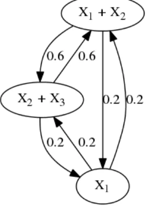
A simple example illustrating the notion of complex balanced equilibrium Let us consider the kinetic system defined by the following four reactions

2X₁ κ₁

GGGGGGAX₂; X₂ κ₂

GGGGGGA2X₁; X₂ κ₃

GGGGGGAX₃; X₃ κ₄

GGGGGGA2X₁. (2.16) The corresponding differential equations are

x˙₁(t) =−2κ₁x²₁(t) + 2κ₂x₂(t) + 2κ₄x₃(t), x˙2(t) =κ1x²₁(t)−κ2x2(t)−κ3x2(t), x˙3(t) =κ3x2(t)−κ4x3(t).

(2.17)

The system (2.17) has an equilibrium at x=

1 κ1

κ₂+κ₃

κ1κ3

κ₄(κ₂+κ₃) T

. (2.18)

The equilibrium point (2.18) fulfils the condition of complex balance which in this case has the form

κ₁x²₁=κ₄x₃, κ₂x₂+κ₃x₂=κ₁x²₁, κ₄x₃=κ₃x₂.

(2.19)

Therefore, the equilibrium point (2.18) is complex balanced.

Deficiency δ is a fundamental property of a reaction network and it is defined as [26]:

δ=m−l−s, (2.20)

where m is the number of complexes (vertices) in the reaction graph, l is the number of linkage classes (graph components) and s is the rank of the reaction network. Another

(18)

equivalent definition of deficiency [15] is

δ= dim(ker(Y)∩im(D)), (2.21)

where Y is the complex composition matrix andD is the incidence matrix of the reaction network. It is easy to see from (2.20) and (2.21) that deficiency depends only on the complex composition matrix and the network structure (i.e. on the unweighted reaction graph), but not on the values of the reaction rate coefficients. The deficiency is a very useful measure for studying the dynamical properties of reaction networks and for establishing parameter- independent (at least) local stability conditions.

It is important to remark that weak reversibility, complex balance and deficiency are all realization-dependent properties and are not the inherent properties of the kinetic differential equations [40, 1]. This structural non-uniqueness will be utilized for realization computation in Chapter 3 and for feedback design in Chapter 4.

2.5 Qualitative dynamical properties of kinetic systems

A central problem of the kinetic systems is the relation between the network structure/

parametrization and the qualitative properties of the dynamics. From the numerous results and conjectures in the field, we only mention those that are directly related to this thesis.

According to theGlobal Attractor Conjecture, for any complex balanced kinetic system its equilibrium pointxis a global attractor in the positive stoichiometric compatibility class S_x [21]. Important special cases were proven in [14] and [63]. Moreover, the possible general proof of the conjecture has recently appeared in [20].

A fundamental result of the kinetic systems is the Deficiency Zero Theorem (Theorem 6.1.1 in [26]) that states the following

(i) If the network is not weakly reversible then, for arbitrary kinetics (not necessarily mass action), the differential equations for the corresponding reaction system cannot admit a positive steady state.

(ii) If the network is not weakly reversible then, for arbitrary kinetics (not necessarily mass action), the differential equations for the corresponding reaction system cannot admit a cyclic composition trajectory along which all species concentrations are positive.

(iii) If the network is weakly reversible then, for mass action kinetics (but regardless of the positive values the rate constants take), the differential equations for the corresponding reaction system have the following properties: There exists within each positive stoichiometric compatibility class precisely one steady state; that steady state is asymptotically stable; and there is no nontrivial cyclic composition trajectory along which all species concentrations are positive.

(19)

Part (iii) is proved by a known logarithmic Lyapunov function that is also independent of the rate coefficients and it has the form

V(x) =

n

X

i=1

x_i(ln(x_i)−ln(x_i)−1) +x_i, (2.22) where x is an equilibrium point. To connect the complex balance and the deficiency zero weak reversibility condition, we also recall from [36] and [28] that a mass action reaction network is complex balanced for any positive choice of rate constants if and only if it is weakly reversible and has a deficiency of zero.

2.6 Dynamically equivalent and linearly conjugate realiza- tions

It is a known result of kinetic systems that a reaction graph corresponding to a given set of kinetic ODEs is generally not unique [22, 53]. Moreover, the kinetic realizability of a polynomial dynamical system is not coordinate-independent and it is preserved only up to the reordering and positive rescaling of the state variables [25].

Based on the above, a kinetic realization (Y, A⁰_k) is called dynamically equivalent to a kinetic system of the form (2.1) if A⁰_k is an m×m Kirchhoff matrix, and Y ∈ Z^n×m₊ such that

M·ϕ(x) =Y ·A⁰_k·ψ(x), ∀x∈Rⁿ+. (2.23) We note that the vector functions ϕand ψare not necessary identical, since the monomials corresponding to product complexes without any outgoing reaction do not appear in the kinetic differential equations.

Therefore, the concept oflinear conjugacy was introduced in [39] that allows a positive diagonal transformation between the solutions of two kinetic systems. For our purposes, it is useful to introduce linear conjugacy in a slightly different way than it was described in [39]. For this, let us perform a state transformation on the kinetic model (2.1) as follows:

z(t) =T·x(t), (2.24)

where T = diag(c) with c ∈Rⁿ₊. Then the differential equations of the transformed model are given by

z(t) =˙ T·M ·ϕ(T⁻¹z(t)) =T·M·diag(ϕ(c))⁻¹·ϕ(z(t)). (2.25) Based on the above calculation, a kinetic realization (Y, A⁰_k) is calledlinearly conjugate to a kinetic polynomial system of the form (2.1) if there exists an n×n positive definite

(20)

diagonal matrix T = diag(c) withc∈Rⁿ₊ such that

T ·M·diag(ϕ(c))⁻¹·ϕ(z) =Y ·A⁰_k·ψ(z), ∀z∈Rⁿ+, (2.26) where Y ∈Z^n×m₊ and ψj(x) =x^Y^·,j forj = 1, . . . , m. The matrix A⁰_k is anm×m Kirchhoff matrix. When we assume that ψ(x) = ϕ(x) for all x ∈ Rⁿ and using the notation A_k = A⁰_k·diag(ψ(c)), we can rewrite (2.26) as follows

Y ·A_k=T ·M, (2.27)

where A_k is a Kirchhoff matrix, too, obtained by scaling the columns of A⁰_k by positive scalars. Therefore, Ak encodes the same reaction graph structure as A⁰_k. This implies that the weak reversibility and zero deficiency properties of the kinetic realizations (Y, A_k) and (Y, A⁰_k) are equivalent. It is also clear that Eq. (2.27) is a linear constraint with respect to Ak and the diagonal elements ofT. Therefore, instead of A⁰_k, we will use the scaled matrix A_k for representing and computing linearly conjugate realizations.

2.7 Computing linearly conjugate realization using optimiz- ation

In this section, we are going to present how one can solve the problem of computing linearly conjugate realizations with optimization methods. For this we choose the problem of computing of the sparse and dense realizations [53]. Sparse realizations have minimum number of edges and a dense realization has maximum number of edges.

Let us consider the polynomial system (2.1). In the realization computation problem the matrixM andϕ(x) are given. The goal is to compute a realization (Y, A⁰_k) with the desired properties (e.g. weak reversibility, zero deficiency) and a diagonal transformationT.

Our optimization based methods assume that the monomials vectorϕ(x) contains all the necessary monomials for the realization computation problem, soϕ(x) =ψ(x) for allx∈Rⁿ and ψ(x) is generated by the fixed complex composition matrix Y. Note that the using of different complex sets results different realizations. Moreover, it is possible that the system (2.1)does not have realization with one set of complexes but it has a realization with another set of complexes. The canonical method [35] always constructs a realization for the system (2.1) when the condition (2.9)is fulfilled. Therefore, it can be used for generating a suitable initial set of complexes but no exact method exists for determining the set of complexes to a given problem.

In the optimization problems we will use a fixed complex composition matrix Y to the linearly conjugate constraint (2.27) that remains linear as a consequence of it. We are going to use decision variables A_k to represent the Kirchhoff matrix of the realization and T = diag([c₁. . . c_n]) to represent the diagonal transformation. First, we have to guarantee

(21)

the linear conjugacy as follows

diag([c₁. . . c_n])·M =Y ·A_k, c_i >0, i= 1, . . . , m,

(2.28)

where M contains the coefficients of the monomials in the polynomial ODE (2.1) that are given real numbers. Note that the LP framework does not handle strict inequalities.

Therefore, the constraints ci >0 can be replaced with ci≥for all i= 1, . . . , n where is a small positive number. Constraints of the Kirchhoff property are the following:

1^TA_k= 0,

[A_k]_i,j ≥0, i, j= 1, . . . , m, i6=j. (2.29) We can introduce a binary matrix variable Θ∈ {0,1}^m×msuch that Θ_i,j is 0 when [A_k]_i,j = 0 otherwise Θ_i,j is 1. This property can be given by linear inequalities as follows

·Θ_i,j ≤[A_k]_i,j ≤U·Θ_i,j, (2.30) whereis a small positive constant andU is the upper bound of values [A_k]_i,j. To reach the maximal (minimal) number of edges we have to maximize (minimize) the following objective function:

X

i,j

Θ_i,j. (2.31)

The constraints (2.28)-(2.30) together with the objective function in (2.31) form a standard mixed integer linear programming (MILP) problem. Note, that the maximization of (2.31) corresponds to determining a dense realization, while minimization finds the sparse realization [53]. Finally, the Kirchhoff matrix of the linearly conjugate realization A⁰_k can be computed as A⁰_k=A_k·diag(ψ(c))⁻¹.

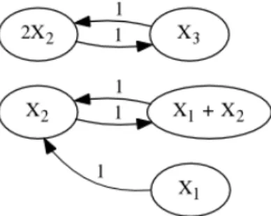
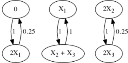
A simple example illustrating the notions of kinetic systems and their realiza- tions Let us consider the following differential equation system in the form

x˙₁(t) =−5x₁(t)

x˙2(t) = 5x1(t)−x2(t) +x3(t)

x˙₃(t) =x₂(t)−x₃(t)−x₁(t)x₂(t)x²₃(t) + 3x₁(t)x₂(t)x₃(t),

(2.32)

(22)

where x_i(t) are the state variables for i = 1,2,3. The system (2.32) has (at least) two different dynamically equivalent realizations. The first one is

x˙ =







1 0 0 1 1 1

0 1 0 1 1 1

0 0 1 1 2 0







| {z }

Y⁽¹⁾







−5 0 0 0 0 0

5 −1 1 0 0 0

0 1 −1 0 0 0

0 0 0 −3 0 0

0 0 0 3 −0.5 0

0 0 0 0 0.5 0







| {z }

A⁽¹⁾_k





 x1

x2

x₃ x1x2x3

x1x2x²₃ x₁x₂







| {z }

ψ⁽¹⁾(x)

. (2.33)

The second one is

x˙ =







1 0 0 1 1 0 1 0 1 1 0 0 1 1 2







| {z }

Y⁽²⁾







−5 0 0 0 0

5 −1 1 0 0

0 1 −1 0 0

0 0 0 −3 1

0 0 0 3 −1







| {z }

A⁽²⁾_k





 x₁ x₂ x3

x₁x₂x₃ x1x2x²₃







| {z }

ψ⁽²⁾(x)

. (2.34)

The realizations (Y⁽¹⁾, A⁽¹⁾_k ) and (Y⁽²⁾, A⁽²⁾_k ) have different complex sets and reaction network structures. The Fig. 2.1. depicts these two realizations, respectively.

(a) Realization (Y⁽¹⁾, A⁽¹⁾_k ) (b) Realization (Y⁽²⁾, A⁽²⁾_k )

Figure 2.1. Two different dynamically equivalent realizations of (2.32). Figures use of the notations of Section 2.2.

(23)

2.8 State feedback control of polynomial systems

Controllers are (possibly dynamical) external systems connected to the one to be controlled (the original or open-loop system) that are designed to achieve a control aim (or control goal) related to the dynamical behaviour of the original system by manipulating through its inputs (see e.g. [38]). The closed-loop system is a composite system consisting of the original system and its controller.

If the controller uses the state of the original system to compute its input, then a state feedback controller is considered. State feedback controllers are widely applied in control theory, because of their efficiency in both achieving stability of the closed-loop system (stabilizing controllers) and ensuring suitable control performance (for example disturbance rejection).

For the purpose of formulating the stabilizing state feedback controller design problem for nonnegative polynomial systems, one needs to consider the input-affine version of Eq.

(2.1) as follows

x˙p(t) =fp(xp(t)) +gp(xp(t))up(t), (2.35) where x_p(t) ∈Rⁿ^p is the state variable, u_p(t) ∈ R^r^p is the input variable, f_p :Rⁿ^p 7→ Rⁿ^p and gp:Rⁿ^p 7→Rⁿ^p^×r^p are polynomial mappings. We are looking for a dynamic polynomial feedback controller in the form

x˙_c(t) =f_c(x_p(t), x_c(t)), u_p(t) =k(x_p(t), x_c(t)), (2.36) where xc(t) ∈Rⁿ^c is the state of the controller, fc :Rⁿ^p⁺ⁿ^c 7→ Rⁿ^c and k :Rⁿ^p⁺ⁿ^c 7→ R^r^p are polynomial mappings. Then, the closed loop system has the form

"

x˙_p(t) x˙c(t)

#

=f(xp(t), xc(t)) =

"

f_p(x_p(t)) +g_p(x_p(t))k(x_p(t), x_c(t)) fc(xp(t), xc(t))

#

. (2.37)

The closed loop system is polynomial, and it is nonnegative if and only if the mapping f is essentially nonnegative. The goal of the feedback control is transforming the open loop system into a closed loop system which has desired properties (e.g stability, performance, etc.).

(24)

Chapter 3

Computing zero deficiency

realizations of kinetic systems

As it has been already discussed in Chapter 2, important model properties such as deficiency, strong connectivity (also called weak reversibility), complex or detailed balancedness are realization dependent but they have strong implications on the qualitative dynamic properties of the kinetic system. Therefore, finding dynamically equivalent or linearly conjugate kinetic system structures with certain required properties is an interesting and important problem for proving qualitative properties of the model.

It was shown earlier that several sub-problems of finding realizations with prescribed properties can be successfully solved in the framework of linear and mixed integer linear programming (see, e.g. [53, 54]). In [40] a MILP-based procedure was proposed for finding weakly reversible linearly conjugate realizations of kinetic systems with minimal deficiency.

The algorithm was based on the result that for weakly reversible realizations, maximizing the number of reaction graph components minimizes the deficiency. This method uses integer variables for the partitioning of complexes between linkage classes. However, it is known that MILP problems are generally NP-hard and therefore it is often computationally problematic to solve large problems containing integer variables. Moreover, for general non- weakly reversible kinetic system structures, the basic principle of [40] can not be applied.

Therefore, the approach of this chapter is chosen to be different, and the aim is to examine and use the special algebraic consequences of zero deficiency to give a general algorithm for computing such realizations of kinetic systems.

The structure of this chapter is the following. Section 3.1 contains the main result of this chapter that is an optimization based method for the computation of deficiency zero linearly conjugate kinetic realizations. In Section 3.2 two illustrative examples are shown, while Section 3.3 summarizes the contribution of this chapter.

(25)

3.1 Computing linearly conjugate zero deficiency realizations

In this section, two new optimization problems are introduced to compute realizations with zero deficiency. The first one works in the general case and it can be solved as an MILP problem. The second one finds weakly reversible zero deficiency realizations, and it can be traced back to an LP problem.

The basic setup for the computations in both cases will follow the problem formulation in Section 2.7. The known parameters are the coefficient matrix M of the ODE (2.1) and the used complex (monomial) set represented by the matrix Y. The decision variables to be computed are the scaled Kirchhoff matrix A_k of the linearly conjugate realization and the diagonal elements of the transformation matrix T. Additional auxiliary constants and decision variables (defined later) will also be used to solve the optimization problems.

3.1.1 Alternative conditions for zero deficiency

In this subsection, equivalent forms of the zero deficiency condition will be given that can directly be used in the framework of optimization.

The next theorem can be found as Lemma 5.8 in [27].

Theorem 1. Let Y andDbe the complex composition matrix and the reaction graph incid- ence matrix of a kinetic system, respectively. Then

dim(ker(Y)∩im(D)) = 0if and only if

R^m = im(Y^T) + ker(D^T). (3.1)

The next theorem was originally published as Corollary 4.11 in [27].

Theorem 2. Let (Y, Ak) represent a kinetic system of deficiency zero. Then ker(Ak) = ker(Y ·A_k).

The following lemma is the immediate consequence of Corollary 4.6 in [27].

Lemma 1. If A_k is weakly reversible thenim(D) = im(A_k).

Using the above results, we can state the following theorem.

Theorem 3. Let (Y, Ak)represent a weakly reversible kinetic system. Then(Y, Ak)has zero deficiency if and only if

ker(A_k) = ker(Y ·A_k). (3.2)

Proof. ⇒ Let us suppose that (Y, A_k) is a weakly reversible kinetic system with zero deficiency. Then, by Lemma 1 we have that im(D) = im(Ak). Substituting Ak into (2.21), we obtain that ker(Y)∩im(A_k) =0, from which it follows that ker(A_k) = ker(Y ·A_k).

(26)

⇐ Now, let us assume that A_k is weakly reversible and ker(A_k) = ker(Y ·A_k). The latter implies that

ker(Y)∩im(Ak) =0. (3.3)

Due to weak reversibility, we can apply Lemma 1 and substitute im(D) for im(A_k) in (3.3).

From this, we obtain that ker(Y)∩im(D) =0that is equivalent to zero deficiency according to Eq. (2.21).

3.1.2 Computing linearly conjugate realizations with zero deficiency in the general (not necessarily weakly reversible) case

In order to put the zero deficiency property into the linear programming framework, we are going to reformulate Eq. (3.1) to the form of linear inequalities.

Eq. (3.1) is fulfilled if and only if there exist vectors y^(`)∈im(Y^T) and η^(`) ∈ker(D^T), such that an arbitrary basis{y˜^(`)} of ker(Y) can be constructed as

y˜^(`)=η^(`)+y^(`), `= 1, . . . , m−rank(Y). (3.4) Let us use the notation W = im(Y^T) + ker(D^T). Clearly, if (3.1) holds then ker(Y)⊂W, and therefore any basis of ker(Y) can be constructed according to Eq. (3.4). Assume now that an arbitrary basis of ker(Y) can be written as in Eq. (3.4). Then ker(Y)⊂W. Since by construction im(Y^T)⊂W, and im(Y^T) is the orthogonal complement of ker(Y), we obtain that R^m= im(Y^T) + ker(Y)⊆W. Recall thatW ⊆R^m, therefore W =R^m.

Since the matrixY is a priori given and constant, we can easily determine a basis{˜y^(`)} of ker(Y). We can also generate an arbitrary element of im(Y^T) with the linear combination of the column vectors of Y^T as follows:

y^(`) =Y^T ·α^(`), (3.5)

where α^(`) ∈Rⁿ.

Clearly, a vector η^(`) is in the kernel of the matrixD^T if and only if

D^T ·η^(`)=0. (3.6)

Since D depends on A_k (i.e. it depends on the reaction graph of the realization), (3.6) is nonlinear in the optimization variables. Therefore, we will use the special structure of the matrix D to convert Eq. (3.6) to an equivalent form which can be inserted into MILP framework. Using the structure of the incidence matrix D, we can state the following theorem.

Theorem 4. Eq. (3.6)can be equivalently represented by the following logical expression:

[A_k]_i,j >0 =⇒ η^(`)_i =η_j^(`), i, j= 1, . . . , m. (3.7)