Introduction to Practical Biochemistry

(1)

(2)

Introduction to Practical Biochemistry

György Hegyi József Kardos Mihály Kovács

András Málnási-Csizmadia László Nyitray

Gábor Pál László Radnai Attila Reményi

István Venekei

(3)

2 Introduction to Practical Biochemistry

by György Hegyi, József Kardos, Mihály Kovács, András Málnási-Csizmadia, László Nyitray, Gábor Pál, László Radnai, Attila Reményi, and István Venekei

(4)

3

Foreword

by Attila Reményi

The ―Introduction to Practical Biochemistry‖ e-book is mainly intended for B.Sc. students studying biology at Eötvös Loránd University. It is part of the course material for students attending the seminars run under the same title. As it covers a broad range of subjects on the basic as well as the practical aspects of biochemical and molecular biological work, it is likely that it will be also useful for any student attending different theoretical or practical biochemistry courses. The course material builds on pre-existing knowledge obtained at previous B.Sc. courses including General Chemistry, Physical Chemistry and Organic Chemistry. It assumes a solid background and experience in chemical calculations and the successful completion of the course entitled ―Introduction to Biochemistry‖, which is taught as part of the Biology B.Sc. program at Eötvös Loránd University, or that of another Biochemistry course at a similar level. The

―Introduction to Biochemistry‖ e-book can be found here.

The ―Introduction to Practical Biochemistry‖ seminar series will prepare students for more advanced courses including the lectures on ―Biochemistry and Molecular Biology‖, and it is particularly indispensable for the third-year hands-on training course entitled ―Practicals in Biochemistry‖. The format of the course may be described as a ―practical seminar‖. This is a mixture of the classical seminar where the theoretical principles are further discussed interactively with students, and the classical practical where the same is accomplished by performing experiments and analyzing experimental data in a first-hand manner. On practical seminars, teachers present the basic principles of techniques broadly used in the biochemical and molecular biological laboratory practice, make some demonstrations on different techniques and show the use of some of the everyday laboratory instrumentation. We have put special emphasis on presenting demonstrations and problem sets that will make the students face ―real-life‖ laboratory situations. Problem sets and biochemical calculations are to be solved interactively, with students working in groups on finding the solution and the teacher being involved only as a discussion moderator.

The e-book is not the description of different biochemical practicals, and it does not contain detailed experimental protocols to perform experiments. It rather contains a collection and description of principles that will help the students perform successful biochemical and molecular biological experiments on their own during their future carrier. The experience of the author team gathered during five years of practice resulted in a course material that enables students to efficiently use hands-on practicals in biochemistry and molecular biology later during their training. Moreover, the material also provides a solid background in biochemical calculations, a prerequisite for successful experimental design.

The e-book covers the course material for a one-semester B.Sc. course delivered in three hours per week. The course does not discuss all families of molecules that are subject to biochemical and molecular biological investigation. It mainly deals with techniques used to study proteins and nucleic acids. The methods on carbohydrates and lipids are discussed as parts of Organic Chemistry courses, and they are also discussed in lectures on ―Biochemistry and Molecular Biology‖.

(11)

10

By completing the ―Introduction to Practical Biochemistry‖ course, students will acquire practical knowledge regarding the techniques used to investigate the properties of macromolecules. As mentioned earlier, the course puts a great emphasis on demonstrating how to solve ―real/life‖ tasks and problems faced by the investigator in biochemical and molecular biological laboratories. Students will become familiar with commonly used labware and instrumentation of a biochemical and molecular biological laboratory, learn the requirements for sterile work, and will be able to store biological samples properly. They learn how to correctly use biochemical units of measure and to make solutions and buffers for basic biochemical experiments. They will be able to determine the charge of weak acids, bases and macromolecules by taking into account their chemical environment. They learn how to measure the macromolecular concentration of solutions by spectrophotometry. They will be able to design protocols for the purification of proteins from cell cultures or tissues. They will become familiar with the physico-chemical background of enzyme action and the fundamentals of enzyme kinetics. They learn how to characterise the interaction between macromolecules and their ligands quantitatively. They will become familiar and be capable of using basic recombinant DNA techniques for nucleic acid manipulation and the production of proteins. They will be able to use public bioinformatics databases to acquire information on the physical, chemical and biological properties of macromolecules.

The e-book comprises 11 chapters dealing with different topics. In addition, Chapter 12 contains more than 100 simple and more complex problems enabling students to constantly put their knowledge to a test by attempting to solve the problem sets belonging to specific chapters.

The author team of the Department of Biochemistry at Eötvös Loránd University wishes the students and all readers an enjoyable experience in entering the field of biochemical and molecular biological laboratory life!

(12)

11

1. Common laboratory tools and equipment used in biochemistry and molecular biology

by László Radnai

The aims of biochemical and molecular biological research are complex and diverse.

Investigation of the network of chemical reactions taking place in living organisms and representing the most fundamental phenomena of life, identification of the molecules playing roles in biochemical processes, determination of their structure, function and interactions, examination of the molecular background of metabolism, the flow of energy and information within organisms are all among the common goals of biochemists and molecular biologists. In accordance with this diversity of problems, a high variety of tools, instruments and methods are required to answer scientific questions effectively. This chapter reviews the most common tools and instruments used very frequently in almost every laboratory. The appropriate handling and storage of biological samples and other chemical substances required for research will also be discussed.

1.1. Biological samples and chemical substances in the laboratory

Tissue or cell samples from a living organism, different cell cultures grown in a laboratory incubator under controlled conditions, homogenates or extracts of cells and tissues, solutions of isolated and purified components (e.g. proteins, nucleic acids) can all be referred to as ―biological samples‖. As the medium of life is water, the majority of biological samples can be defined as aqueous solutions with one or more components, colloidal systems, or water-based suspensions (e.g. bacterial cells dispersed in a liquid medium). Consequently, most biochemical experiments also take place in aqueous environments. Therefore, laboratory vessels used to store liquids and laboratory tools required for the manipulation, transfer and accurate volume measurements of liquids will be introduced in this chapter. Different solids (e.g. chemical substances obtained from different companies, synthetic oligonucleotides or peptides) are also often necessary for biochemical research. In most cases, solids are dissolved in water (or sometimes in other solvents) prior to the experiments. Therefore, the methods of preparing solutions and measuring accurately the weight of the required solids will also be discussed below. Sometimes we use gases in the laboratory. These can be stored in gas cylinders (e.g. O2), in Dewar flasks in liquid state (e.g. liquid nitrogen), or dissolved in water (e.g. HCl or NH3). By working with gases it is very important to follow all safety instructions to avoid fire, explosions, frostbite or (in case of inhalation) asphyxia or poisoning.

1.2. Plastic and glass tubes used for the storage of liquids

Vessels made of different transparent plastics are widely used in laboratory practice for the storage of liquids. Plastics are cheap and flexible. Containers, flasks and tubes are often equipped with lids, caps, or screw-caps. Moreover, plastic containers are ideal because they retain their flexibility in a wide range of temperatures, while glass can be more sensitive to temperature changes or can be broken easily. For the storage of liquids, probably the most important criterion

(13)

12

is the air-tightness of the vessels. An air-tight cap can protect the sample from the evaporation of the solvent. It also protects against dust, bacteria, mould spores or other impurities originating from the environment. It blocks the dissolution of different gases into the sample. Dissolved gases can modify the biomolecules directly (e.g. oxygen reacts with sulfhydryl groups of cysteines within a protein, leading to the formation of disulphide bonds) or indirectly (e.g. carbon dioxide forms carbonic acid in water, which dissociates and decreases the pH of the solution, thereby affecting the protonation state and solubility of proteins). Plastics have some other advantages. One of these is their inertness against the majority of chemical substances used in most experiments. However, some experiments may require the use of organic solvents. In such cases one needs to check the compatibility of the given solvent with the plastic vessels prior to the experiment.

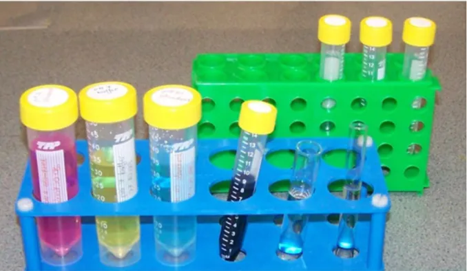
Liquid samples with volumes up to 50 millilitres can be stored in so-called Falcon tubes (also called Falcon centrifuge tubes) (Figure 1.1). Falcon tubes are manufactured with different nominal volumes (most typically, 15 mL and 50 mL) and are supplied with screw-caps. The conical bottom of the tube is particularly advantageous when there is only a small amount of liquid left in the tube. In this case all drops can be collected readily by centrifugation. These tubes have to be placed into appropriate racks. However, there are also free-standing tubes available having a plastic ―skirt‖ around the conical bottom. These tubes can be placed on horizontal surfaces without any support, but must be handled carefully to avoid tipping up. Falcon tubes are graduated; thus the volume of the sample can be estimated easily. However, more precise volumetric measurements require other laboratory tools (e.g. graduated cylinders). It is crucial in all laboratories to mark the samples unambiguously. Unlabelled samples are generally (and rightfully) considered as litter. Falcon tubes can be labelled on the top of the screw-caps or on the side of the tube. (They often have an area with white background for this purpose.) Labels can be printed or hand-written by using a marker pen. Illegible writing must be avoided and the label must be protected against abrasion, e.g. by a piece of transparent cellophane tape. Components of the sample, concentrations, solvent(s), buffering component(s) and pH, possible toxicity are the most important parameters that generally need to be indicated on tubes. The name of the experimenter and/or the date of the sample preparation or the experiment are also often important, especially if the components are prone to degradation.

(14)

13

Figure 1.1. 50-mL and 15-mL Falcon tubes, glass test tube and Wasserman tube (left to right in blue rack) in plastic racks.

Test tubes and narrower Wassermann tubes (Figure 1.1) are usually made of glass and provided without caps. They have a U-shaped bottom. They are mainly used for temporary purposes (e.g.

for preparing reaction mixtures or for collecting fractions during chromatographic separation of different components). The main advantage of glass is its high resistance against most chemical substances and solvents used in typical biochemical experiments (with the exception of concentrated strong bases). If the long-term storage of the sample is necessary, the openings of the tubes can be closed air-tightly by a piece of parafilm (Figure 1.2). Parafilm is a thin layer of paraffin, manufactured and supplied with a paper backing. It is ductile, flexible and cohesive. The opening of the test tube (or other laboratory container) can be covered by using a piece of parafilm of appropriate size. Overhanging ends must be wrapped around the neck tightly.

Parafilm is often used also to provide additional sealing on laboratory vessels and tubes having a cap or lid, in order to protect the sample more effectively.

(15)

14

Figure 1.2. A, One roll of parafilm in a dispenser box. B, Cutting a piece of parafilm with scissors. C, Removal of the parafilm layer from the paper backing. D, Covering a Wasserman tube with a piece of parafilm. E, Wrapping the overhanging ends around the opening of the tube.

F, Wasserman-tube sealed with parafilm. G, Parafilm ensures air-tight sealing.

For samples of small volume (ranging from several microlitres to several millilitres), Eppendorf tubes (or Eppendorf microcentrifuge tubes) are used (Figure 1.3). These tubes are available in different nominal volumes (e.g. 0.5 mL, 1.5 mL, 2 mL and 5 mL). The most common size is 1.5 mL. Eppendorf tubes have a conically-shaped bottom. Hence, they need to be placed in appropriate plastic racks. They are equipped with an attached plastic snap-lid. The connection between the snap lid and the tube is flexible enough to allow opening and closing many times.

(16)

15

Labels can be placed on etched marking areas on the top of the lid and on the side wall of the tube.

Figure 1.3. Eppendorf tubes with nominal volumes of 0.5 mL (left) and 1.5 mL (top green rack) and PCR tubes with a nominal volume of 200 μl (bottom right corner).

PCR tubes (Figure 1.3) are named after their main purpose of usage, the polymerase chain reaction. PCR is one of the most commonly applied enzymatic reactions in recombinant DNA technology that is used frequently in the majority of laboratories to amplify a specified segment of linear double-stranded DNA. Nominal volumes of PCR tubes typically range up to 200 μl.

Similarly to Eppendorf tubes, PCR tubes are equipped with an attached snap-lid, and have an etched marking area on the top of the lid or on the side wall of the tube. Besides their application in PCR reactions, PCR tubes can be used for a variety of other enzymatic reactions.

1.3. Beakers and laboratory flasks

Beakers (or laboratory beakers) are simple cylindrical vessels with a flat bottom, typically used for the preparation and short-term storage of solutions and liquids (Figure 1.4). Nominal volumes of beakers vary between a few millilitres and several litres. Beakers are usually made of glass or plastics and are graduated, aiding the estimation of the actual volume of the sample. However, precise volumetric measurements are not possible with beakers. Beakers made of heat-shock resistant borosilicate glass are suitable for the heating or boiling of solutions by using a Bunsen burner.

(17)

16 Figure 1.4. Glass and plastic beakers of different size.

A variety of flasks are widely used in laboratories, mainly for the storage and preparation of solutions. Some flasks are used with silicone or rubber stoppers, some have standard taper joints equipped with glass stoppers that fit tightly into the opening. Other flasks can be sealed by using a piece of parafilm. Nominal volumes of flasks typically vary between 50 millilitres and several litres. Like beakers, laboratory flasks can be made of glass or plastics. Precise volumetric measurements can only be performed by using volumetric flasks; however, this special subtype is rarely used in biochemical laboratories. The most commonly used flask is the so-called Erlenmeyer flask (also known as conical flask) (Figure 1.5), which has a conical body, a wide and flat bottom and a narrow neck. It is especially suitable for growing bacterial (or eukaryotic) cells in nutrient liquid media inside an incubator at a controlled temperature (Figure 1.5, panel B). Incubators provide continuous shaking of cultures to prevent sedimentation of cells and facilitate gas exchange (oxygen is required for efficient growth), also supported by the shape of the Erlenmeyer flask. (The surface of the liquid is relatively large due to the wide bottom of the Erlenmeyer flask.) The wide and flat bottom also helps in fixing the flasks into the holders of the plate of the incubator, while the narrow neck prevents the culture from spilling out. Openings are covered by a piece of aluminium foil allowing gas exchange while keeping out dust, other bacteria or spores from the environment.

(18)

17

Figure 1.5. A, Erlenmeyer flasks. B, E. coli bacteria growing in Erlenmeyer flasks.

1.4. Precise volumetric measurements with graduated cylinders and micropipettes

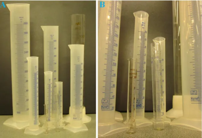
Graduated cylinders (Figure 1.6) are used to measure the volume of liquids precisely, ranging from a few millilitres to several litres. These laboratory vessels are essential for mixing or dispensing different liquids and for the preparation of solutions with pre-defined concentrations and volume. They are available in many different sizes ranging from 5 millilitres to a few litres.

(19)

18

Figure 1.6. A, Glass and plastic graduated cylinders of various sizes. B, Small graduated cylinders (10 - 100 mL, middle of image).

While the smallest graduated cylinders can be used to measure volumes as small as 5 millilitres, it is often necessary—especially in biochemical and molecular biological work—to extend the range of accurate volumetric measurements below 1 millilitre or even below 1 microlitre.

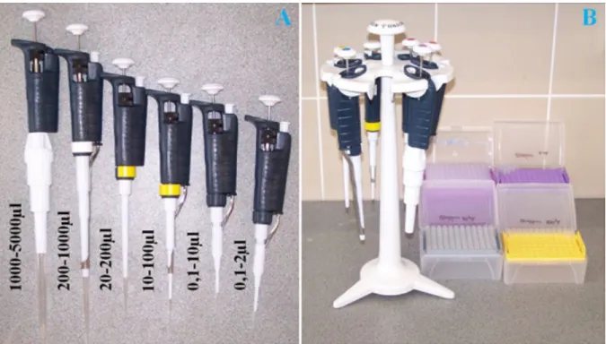
Micropipettes (also called piston-driven air displacement pipettes) are the most common laboratory tools applicable in this volume range (Figure 1.7). Within the plastic body of a micropipette, a piston is operated by pushing a button on the top of the device. The button is connected to the piston through a metal rod. The downward movement of the button causes higher pressure inside the airtight cylinder of the piston, thereby pushing out air from the device through a long, hollow plastic shaft, while upward movement generates vacuum. The vacuum is used to draw up liquid into a removable transparent plastic tip. Tips must be fixed in an air-tight manner onto the end of the plastic shaft of the pipette. Without an air tight connection, the volume being drawn will be reduced and undesired leakage will occur during the transfer of the liquid. Disposable tips are used to avoid cross-contamination of samples and stock solutions. Tips must be changed after each operation. (The synthesis and/or purification of chemical substances, proteins, enzymes, nucleic acids and other samples can be extremely laborious, time-consuming and expensive. Therefore, the avoidance of contamination is a crucial issue. Contaminated samples must be discarded and must not be used for any further experiments.) The desired pipetting volume can be set on the pipette, causing a controlled restriction of the movement of the piston. This can be done by turning the volume adjustment knob on the side of the pipette.

(20)

19

(Alternatively, the plunger button of several pipettes is used for volume adjustment purposes.) The actual volume is indicated on a digital volume indicator on the side of the pipette body.

Maximal and minimal allowed volumes are also indicated on the body or on the top of the pipette. Setting volumes beyond these limits should not be attempted because such operations will damage the pipette and lead to significant inaccuracies. There are pipettes available for different volume ranges. Large pipettes can be used between 1 mL and 5 mL. Below 1 mL, there are several pipettes with the following typical ranges: 200 µL - 1000 µL, 20 µL - 200 µL, 10 µL - 100 µL, 5 µL - 50 µL, 2 µL - 20 µL and 0.5 µL - 10 µL. The transfer of as little as 0.1 µL of liquid is possible with the smallest pipettes with a typical range of 0.1 µL - 2 µL.

Figure 1.7. A, Micropipettes for different volume ranges. B, Pipettes hanging on a rotating pipette stand, and different tips in racks.

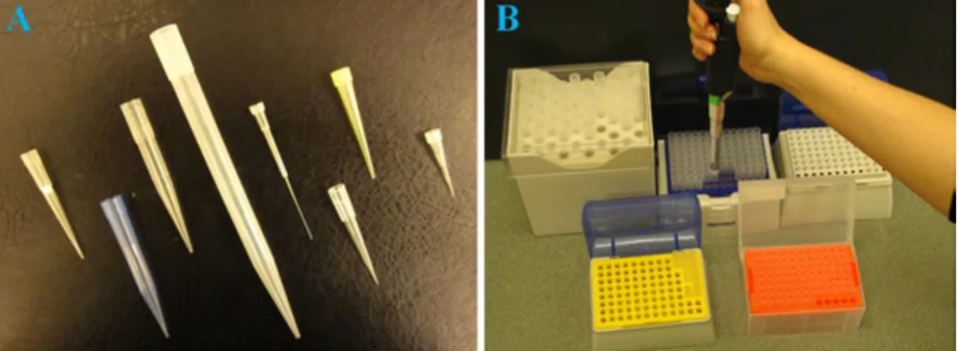
Different tips can be obtained from suppliers according to the volume range of the pipette. Tips can also meet some special criteria, e.g. there are tips supplied with an inner filter for sterile work, or long and narrow tips being very useful in situations where the bottom of deep and narrow tubes or wells must be reached (Figure 1.8). As tips are made of transparent plastics, the operation of the pipette can easily be checked by visual inspection (e.g. for the presence of undesired air bubbles entering the tip together with the liquid, which will cause inaccuracies).

Tips can be removed from the shaft of the pipette by pushing the tip ejector button. This button is connected to a long arm surrounding the shaft and transmitting the force towards the upper end of the tip. Tips are also available pre-packed in appropriate racks. Racks protect tips from contamination and facilitate the fastening of the tips onto the pipette (Figure 1.8, panel B). (The shaft of the pipette can simply be pushed into the upper part of the tip.)

(21)

20

Figure 1.8. A, Pipette tips suitable for different pipettes and purposes (e.g. tips with sterile filters or elongated tips). B, Fastening of a tip onto the pipette.

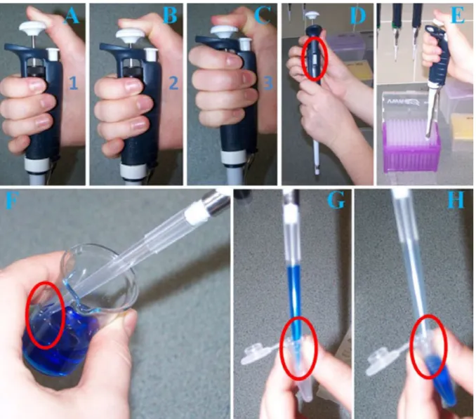
Micropipettes are user-friendly laboratory devices. However, the desired pipetting accuracy can only be achieved by some practice (Figure 1.9, panels A-H). The button of the pipette (and the connected piston) has three characteristic positions (Figure 1.9, panels A-C). In the resting position, the button is pushed up by a spring (first position). By pushing the button gently down with one‘s thumb (exerting a moderate force on it), air will leave through the previously fixed tip.

The button stops in the second position when the desired volume (the one that has been set by the volume adjustment knob) has been reached. While holding the button in the second position, the end of the tip must be submerged into the solution and, subsequently, the button must be released very slowly to let the piston return to the first (resting) position, thereby drawing the desired amount of liquid into the tip. The liquid can then be transferred to another location (e.g. into a test tube or other vessel). Pushing down the button again to the second position will release the liquid.

However, a drop often remains at the end of the tip. To avoid inaccuracies, the entirety of the pipetted solution can be removed by exerting a higher force on the button and pushing it down to the third position. This way, some extra air will be blown out through the tip, thereby removing the remnants of the pipetted liquid. The button must not be released until the tip has been raised above the surface of the solution. (For complete removal of the remaining drop, the tip can be pulled out while the button is being pushed from the second to the third position.) The pipette must be held in a vertical position (with the tip pointing downwards) while transferring liquids.

Tilting of the pipette may cause the liquid to leak into the inner parts of the device, causing corrosion and/or contamination. To prevent this, some pipettes have an inner filter (Figure 1.9, panels F-H). When transferring small volumes (e.g. less than 1 µL of an enzyme solution), only the surface of the liquid should be touched with the end of the tip, as small drops can adhere to the outer surface of the tip and cause significant inaccuracies.

(22)

21

Figure 1.9. A-C, Three positions of the button of the pipette. D-H, Liquid handling with pipettes.

D, Adjusting the volume. E, Fastening an appropriate tip. F, Drawing of the liquid. G, Transferring the liquid into an Eppendorf tube. H, Dispensing the liquid.

1.5. Mixing of liquids

Appropriate mixing of different solutions or liquids is a crucial issue in biochemical experimentation. (Diffusion can be very slow!) Pipettes are perfect tools for mixing volumes not exceeding far beyond their volume range. Submerging the tip into the solution and subsequent pushing and releasing the button (between the first and the second positions) several times will ensure extensive mixing.

The so-called Vortex mixer can be used as an alternative (Figure 1.10, panel A). By pushing down the rubber platform on the top of the device with the bottom of a tube containing the solution to be mixed, the platform will start to oscillate rapidly along a circular path. The liquid will start to shake and swirl along the walls of the tube, ensuring quick and efficient mixing even

(23)

22

if the volume of the solution is very small (e.g. a few microlitres). While vortexing, the tube must be held with fingers approximately at the upper third of its height to avoid splashing out. (The liquid usually stays below the level of one‘s fingers.)

Magnetic stirrers are used for the mixing of large volumes (Figure 1.10, panel B). Magnetic stirrers contain an electric motor that rotates a strong permanent magnet. The angular speed of the motor can be set by a knob. The vessels (e.g. beakers, flasks, graduated cylinders) containing the liquid to be mixed are placed onto the top of the device. Some stirrers are equipped with a heater to warm up the solution. A stirring bar (a rod-like strong magnet with coating made of an inert plastic) is dropped into the liquid. The motion of the stirring bar follows the rotation of the magnetic field. Effective mixing is ensured by the spinning stirring bar within the solution.

According to the volume and the geometry of the vessels, there are stirring bars available in different sizes and shapes (Figure 1.10, panel C). Magnetic stirrers are very useful tools for the facilitation of the dissolution of crystalline or solid chemical substances. They are also used widely if continuous, intensive mixing is necessary. A typical example is the adjustment of the pH of buffer solutions when a digital pH meter is used to continuously monitor the actual pH of the solution during titration with a strong base or acid until the desired pH value is reached.

(Digital pH meters are equipped with a glass electrode that gives a voltage signal proportional to the concentration of oxonium ions in the solution.)

Figure 1.10. A, Mixing of a solution with a Vortex mixer. B, Mixing of a solution with a magnetic stirrer during pH adjustment (the glass electrode of the pH meter is immersed into the solution). C, Stirring bars of different size and shape.

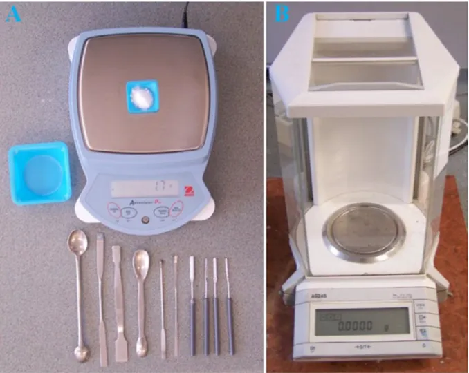
1.6. Laboratory balances

Digital laboratory balances with of different capacity and accuracy are available for the measurements of the weight of samples and chemicals. Top-loading balances typically work with

(24)

23

0.1 g accuracy in the range from several grams to several hundred grams (Figure 1.11, panel A).

For the precise measurement of small weights, analytical balances are used. These devices usually work with 0.01 mg accuracy in the range from 0.1 mg to several grams. A vibration-free, flat and horizontal surface is required for proper operation of such balances—usually a free- standing table with a marble surface plate. Moreover, the convection of the air around the balance should be avoided. (Air currents can exert forces on the pan of the balance comparable to the force exerted by the sample being measured.) For this purpose, analytical balances have a built-in enclosure with doors made of transparent plastic sheets (Figure 1.11, panel B). Measurements can be performed within this protective enclosure. Disposable weighing dishes and laboratory spatulas with spooned ends are important accessories of weight quantification. It is also possible to dispense solids directly into a beaker or a laboratory tube instead of a weighing dish—

however, heavy vessels (with a mass above the upper limit of the balance) must not be applied.

The mass of the empty dish must be determined first. Then, the display of the scale must be set to show zero by pushing the ―tare‖ button. Next, the substance is added into the weighing dish. The display will thus show the pure mass of the substance.

Figure 1.11. A, Top loading balance with disposable weighing dishes, laboratory spatulas and spoons. B, Analytical balance on a vibration-free surface.

(25)

24

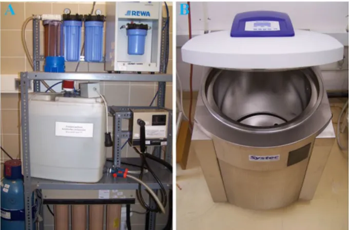
1.7. Methods of sterilisation and in-house production of high-purity water

High-purity water suitable for biochemical and molecular biological experiments is a general need in all laboratories. Distilled or deionised water can be obtained from different suppliers.

However, equipment for its in-house production is also available. Successive distillation is one of the applicable methods. Distillation is energy-consuming and expensive, and it raises various safety issues. A more common alternative is the filtration and deionisation of piped water with a combination of different filters and deionising resins (Figure 1.12, panel A). The applied filters have decreasing average pore diameters; thereby, they gradually remove the corresponding fractions of different contaminating floating particles, microorganisms and bacteria. Deionising resins exchange soluble ions (e.g. calcium, magnesium, sodium, bicarbonate, chloride or heavy metals) for oxonium or hydroxide ions. Clogged filters and used deionising resins must be replaced regularly. The quality of water must be constantly monitored by measuring its electric resistance by conductometers. (The resistance of pure water is above 18 MΩcm at room temperature.)

The importance of using high-purity water, high-quality chemicals and solvents cannot be overestimated. Moreover, having clean laboratory vessels, tubes and devices is also a basic necessity. Some experiments (especially if living cells or organisms are involved) require sterile laboratory vessels and equipment. We consider an experimental setup sterile if microorganisms originating from the environment are removed from it or killed. Depending on the properties of the given sample, chemical substance or device, there are many physical or chemical methods for sterilisation.

Laboratory suppliers sell sterile equipment (Eppendorf tubes, pipette tips, etc.) in sealed sterile bags. However, sterilisation can also be performed in-house, most commonly by using autoclaves (Figure 1.12, panel B). Autoclaves are equipped with a chamber with strong walls in which the process of sterilisation takes place. When all solutions, vessels and other laboratory equipment to be sterilised have been placed inside the autoclave, a defined amount of water must be poured into the chamber. (The objects to be sterilised are standing on shelves or stages so that the water level in the chamber stays below them.) After closing the airtight door, the autoclave starts to heat up the water. Heating the water in a closed system results is the formation of hot steam and elevated pressure. Autoclaving for 20 minutes at 121°C results in sterility by destroying even the highly resistant endospores of bacteria. (In case of overpressure, safety valves are put into action to keep the process under control.) Equipment and chemicals are to withstand the high temperature in the autoclave; therefore, heat resistance must be checked prior to sterilisation.

While laboratory glassware is heat resistant in the applied temperature range, some plastics melt at 121°C. When sterilisation by autoclave is necessary, laboratory tools made of heat resistant plastics must be obtained. Pipette tips must be placed into appropriate racks before sterilisation.

Glassware, Eppendorf and Falcon tubes etc. must be placed into bigger vessels and covered with aluminium foil to avoid contamination after the sterilisation procedure. Solutions can also be autoclaved; however, if there are any components susceptible to thermal decomposition, other methods of sterilisation must be sought. Most inorganic compounds and some simple organic compounds (including typical buffers) are not prone to thermal decomposition at 121°C. Liquid media (e.g. for bacterial cell culture) can also be sterilised in an autoclave.

(26)

25

Figure 1.12. A, Filtration and deionisation of water. B, Autoclave.

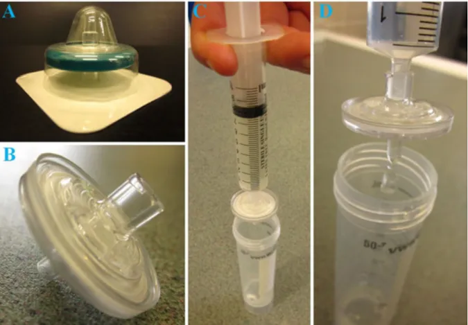
If the thermal stability of the solution is low (when, for instance, glucose or other monosaccharide is present), sterile filtration can be a good alternative to autoclaving. Sterile filters (Figure 1.13) are pre-sterilised filters with pore sizes smaller than the diameter of bacterial cells (0.2 µm). They are packed in separate envelopes to avoid contamination. The solution can be filtered by using a syringe with an appropriate filter fixed onto it, or by using a vacuum chamber with a filter placed into a funnel on the top of the device.

(27)

26

Figure 1.13. A, Sterile filter within its protective envelope. B, Close-up view of a sterile filter. C, Sterile filter fixed onto a syringe. D, Syringe-driven filtration.

1.8. Working with cell cultures

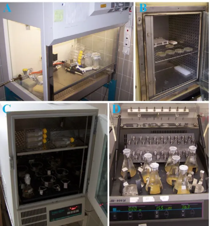
Sterility is a crucial issue during working with different cell cultures. Undesired microorganisms accidentally getting into a solution often start to grow by utilizing and degrading the available components. As these microorganisms synthesise the biomolecules of their cells, they release various metabolites into the solution. (Some algae can grow even in distilled water!) Cell cultures (e.g. the cultures of the E. coli bacterium used widely in recombinant DNA techniques) must be protected from such ―invaders‖. To achieve this, sterile laboratory tools, vessels and media must be used. A laminar flow cabinet (also known as tissue culture hood) is required for most operations performed with cell cultures (Figure 1.14, panel A). In the laminar flow cabinet, a constant air current is established. Air filtered through a HEPA (high-efficiency particulate air) filter is blown into the cabinet at the top, and leaves below the working bench. HEPA filters remove all microorganisms. The transparent door of the cabinet protects its inner contents from contamination. While the door is opened, work can be done through a narrow gap allowing only the hands of the operator to reach the equipment and the cell cultures inside. The operator must wear laboratory gloves. Ethanol and/or a Bunsen burner can be used to quickly sterilise equipment inside (e.g. inoculation loops, glass spreaders). Other accessories, including pipette tips and different tubes, are sterilised in an autoclave prior to use. It is very important to avoid

(28)

27

situations in which the arm of the operator or any non-sterile equipment is directly placed above sterile cell cultures (or any sterile equipment), because dust particles or bacteria transferred by the air flow (pointing downwards) can easily contaminate the sterile components. Upon finishing the desired operations, the front door of the laminar flow cabinet must be closed. The inner contents can be sterilised by using a built-in UV lamp.

Incubators are used to maintain controlled conditions for bacterial or eukaryotic cell cultures (Figure 1.14, panels B-D). These devices can heat or cool their inner space in order to provide constant temperature conditions for cells. (Simpler and cheaper incubators can only heat; hence, these can only be used above ambient temperature.) Cells can be cultured on different surfaces.

Bacteria are often grown in Petri dishes on the top of a layer of gelatinous nutrient agar medium (Figure 1.14, panel B), while eukaryotic (e.g. human) cells are grown at the bottom of cell culture flasks, covered by liquid medium at an appropriate height (Figure 1.14, panel C). Most of the commonly used eukaryotic cells are adherent: they settle and grow while attached to the surface of the cell culture dish.

Besides temperature, the most important environmental factor is the gas mixture in which the cells are being cultured (for instance, obligate anaerobic bacteria are killed by oxygen, and eukaryotic cells often require elevated levels of carbon dioxide). If necessary, a controlled atmosphere can be maintained by using appropriate incubators.

In general, cells grown in liquid cultures (suspended in liquid medium) can reach higher densities than adherent cultures, because in liquid cultures the entire culture volume can be utilised for growth. Liquid cultures are used if cells are required in large numbers (e.g. during recombinant protein expression in E. coli bacteria) (Figure 1.14, panel D). As mentioned above, Erlenmeyer flasks are the most widely used vessels for this purpose. Incubators equipped with a shaking platform are necessary to ensure uniform cell densities and growth conditions within the medium.

Intensive shaking of the flasks by circular motion facilitates effective gas exchange. The attained cell density can be further increased by the use of fermentors.

(29)

28

Figure 1.14. A, Laminar flow cabinet. B, Incubator (37°C) with bacterial cultures on agar plates.

C, Incubator (37°C) with cultures of eukaryotic cells. D, Incubator (37°C) with a shaking platform for liquid cultures of E. coli bacteria (in Erlenmeyer flasks).

1.9. Centrifuges

Cells can readily be harvested from liquid cultures by using different centrifuges (Figure 1.15).

Similarly, any suspension or floating colloidal particles (e.g. precipitated proteins) in a solution can be separated into fractions by spinning the sample in a centrifuge (see also Chapter 5 for

(30)

29

more detail). The resulting fractions are referred to as ―supernatant‖ (i.e. the solution) and

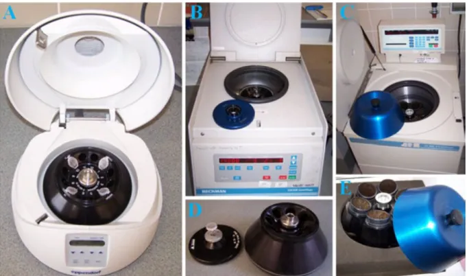
―pellet‖ (i.e. the particles collected at the bottom of the centrifuge tube, pressed together into a compact mass). Centrifuges are relatively simple devices having stationary and rotary parts. The rotation generated by the electric motor of the centrifuge is transmitted to the rotor harbouring the samples contained within appropriate centrifuge tubes. Many biochemical samples are heat sensitive; for instance, proteins denature at elevated temperatures. Such samples require refrigerated centrifuges in which low temperature can be maintained during centrifugation.

Centrifuges are available in different sizes ranging from simple bench-top centrifuges to preparative devices with much higher capacities (volumes up to several litres). Eppendorf tubes or Falcon tubes fit into some rotors of bench-top centrifuges, thereby simplifying the processing of many samples. Most centrifuges can be used in conjunction with several different rotors. This versatility allows users to adapt their centrifuges easily according to the actual requirements.

Centrifuge tubes (Figure 1.16) must be chosen according to the manufacturer‘s instructions.

Importantly, the filled rotor must be counter-balanced during operation. To achieve this, tubes with equal weights must be placed into opposite buckets or holes of the rotor. The weight balance should always be checked by simple two-armed or digital scales. If the weights of the sample tubes are different, counter-balances must be prepared by filling similar tubes with water.

Unbalanced rotors are subject to extremely high forces during rotation. Even a small asymmetry of the weights around the axis of rotation can result in the breakage of the rotor shaft at high angular speeds. In such cases, the rotor may also damage the whole device and even cause serious personal injuries.

(31)

30

Figure 1.15. A, Bench-top Eppendorf centrifuge with samples arranged symmetrically around the axis of the rotor. B, Semi-preparative, refrigerated centrifuge with a rotor for Eppendorf tubes. C, Preparative, refrigerated centrifuge with a rotor for the handling of volumes up to 6 litres. D, Semi-preparative rotor with lid. E, Preparative rotor with lid.

Figure 1.16. Centrifuge tubes.

(32)

31

The rotation speed of centrifuges is often specified as the number of revolutions per minute (RPM). However, as the force applied to the sample depends not only on the actual RPM value but also on the radius of the rotor, the relative centrifugal force (RCF) is more informative about a particular experiment. This defines acceleration according to the mass of particles floating in the sample. Therefore, RCF values are given as relative acceleration values (the centrifugal acceleration compared to g, ~9.8 m/s², the acceleration due to gravity on the surface of Earth).

Thus, if the same sample is spun at equal RPM values in two centrifuges with different rotor geometries (different rotor radii), the results will be different. However, if equal RCF values are applied, sedimentation forces will be identical. Therefore, RPM values are only informative when specified together with the rotor type or radius.

Simple centrifuges can provide maximal accelerations around 10⁴ g. Ultracentrifuges (Figure 1.17) are capable of operating at maximal accelerations in the range of 10⁵-10⁶ g. To reach high angular speeds, ultracentrifuges generate vacuum around the rotor to decrease aerodynamic drag.

Ultracentrifuges can be used for preparative (e.g. removal of cell debris from a lysate prior to the isolation of recombinant proteins) or analytical purposes (e.g. investigation of the interactions or the oligomerisation of different biomolecules). (The reader may remember that the first evidence of the semi-conservative replication of DNA also came from density gradient ultracentrifugation experiments.)

(33)

32

Figure 1.17. A, Micro-ultracentrifuge (RPMmax = 100000 min^-1, RCFmax = 300000 g). B, Rotors compatible with the micro-ultracentrifuge. C, Semi-preparative ultracentrifuge (RPMmax = 70000 min^-1, RCFmax = 350000 g). D, Rotors compatible with the semi-preparative ultracentrifuge.

1.10. Other widely used laboratory techniques: spectrophotometry, electrophoresis, chromatography

One of the most often used instruments in laboratories is the spectrophotometer (Figure 1.18). A photometer is a device measuring the intensity of light after passing through a sample (most often, a solution). Absorption of light by the sample will reduce the measured light intensity. A spectrophotometer is a photometer that can measure the absorbance of the sample at different wavelengths of the light. The absorbance depends on the presence and concentration of absorbing molecules (see Chapter 4 for more detail). Hence, spectrophotometers are widely used to determine the concentration of different biomolecules that show characteristic absorption (e.g.

proteins, nucleic acids). Sample holders used in spectrophotometers are called cuvettes (Figure 1.18; see also Chapter 4). Depending on the wavelength range of the measurements, cuvettes made of transparent plastics, glass or quartz glass may be applicable. Plastic or glass cuvettes can be applied in the range of visible light (they are transparent as they do not absorb visible light).

Quartz cuvettes have low absorption both in the UV and visible range of the spectrum. If the absorbance of many samples needs to be determined simultaneously, plate readers (Figure 1.18, panel C) can be used instead of spectrophotometers. These instruments can dramatically reduce

(34)

33

the required working time. Samples are dispensed into the wells of plastic plates (e.g. those of a 96-well microplate with 8 rows and 12 columns of wells), and subsequently placed into the plate reader. Absorbance readings are transferred to and processed by a computer. Spectrophotometry and spectrophotometers will be discussed in more detail in Chapter 4.

Figure 1.18. A, Spectrophotometer. B, Different types of cuvettes: photometric sample holders made of plastic, glass or quartz. C, Plate reader with samples loaded onto a 96-well microplate.

It is often necessary to isolate and purify one or several components from a solution. Various methods are available for the separation of biomolecules. Electrophoretic and chromatographic methods represent two major families of separation techniques (Figure 1.19).

Charged particles in a homogeneous electric field experience different forces. Positively charged particles are repelled from the positively charged electrode (i.e. the anode), while they are attracted by the negatively charged electrode (i.e. the cathode). Negatively charged particles are attracted by the anode and repelled by the cathode. This phenomenon also appears in aqueous solutions. Electrophoresis (Figure 1.19, panel A) exploits the force exerted by an electric field on a charged biomolecule in solution. (For instance, DNA is negatively charged resulting from the deprotonated state of the phosphate moieties of its sugar-phosphate backbone.) Electrophoretic experiments are carried out in gelatinous substances in which the charged biomolecules can be separated according to the differences in their charge, molecular size and shape. Gels are three- dimensionally cross-linked systems of macromolecules with porous structures. Pores are filled by the aqueous solution. As the pore sizes are comparable to the sizes of molecules to be separated,

(35)

34

smaller molecules migrate faster than large molecules within the gel. This effect is called molecular sieving. (Electrophoretic methods will be discussed in more detail in Chapter 7.) Chromatography is another large family of separation techniques. In chromatography, the components of a mixture (e.g. a solution of biomolecules) are separated based on their differential partitioning between two phases: the so-called stationary and the so-called mobile phase. In biochemistry, the stationary phase is generally composed of small beads of a polymeric substance filled into a column (a tube made of glass, plastic or metal with a filter at the bottom), while the mobile phase (or eluent) is the solution carrying the analyte (i.e. the mixture of substances to be separated) through the stationary phase. Separation can be based on the size, shape, charge, isoelectric point, hydrophobicity or specific binding affinity or biological activity of the compounds. Different stationary phases are available to exploit these molecular features.

The mobile phase must be chosen according to the properties of the sample and the stationary phase. Automated or semi-automated chromatographic systems typically include vessels for different buffers and solvents, pump(s) responsible for the delivery of the mobile phase, an injector responsible for loading the samples onto the column, various chromatographic columns, detector(s) monitoring the composition of the eluate (i.e. the solution leaving the column), a fraction collector, and a computer for controlling the units and analyzing data (Figure 1.19, panels B-C). Chromatography will be discussed in more detail in Chapter 6.

Figure 1.19. A, Power supply and buffer tank for gel electrophoresis. Gels are placed into the buffer tank. B, High-Performance Liquid Chromatography (HPLC) system. C, Fast Protein Liquid Chromatography (FPLC) system.

1.11. Storage of biological samples

Processing or purifying biological samples is often time consuming and labour-intensive. Hence, it is often necessary to store the samples for various time periods. As the samples can be highly divergent (e.g. living eukaryotic cells or bacteria, tissue samples, solutions of proteins or nucleic acids) and show different susceptibility to physico-chemical changes, optimal storage conditions have must be determined in each case experimentally. In an ideal case, the composition, chemical and physical properties and the biological activity of the sample all remain unchanged over time.

(36)

35

Unfortunately, this is never true in practice. Therefore it is very important to optimise storage conditions and minimise the time of storage via good timing of the experiments.

A variety of spontaneous reactions and enzymatic processes can occur in any biological sample at different rates, transforming and/or degrading its key components. Some reactions require the components of air as reagents (for instance, oxygen reacts with sulfhydryl groups of proteins). It is relatively easy to protect the samples from such reactions by using a tube supplied with an air- tight cap, which is especially important during long-term storage. Further protection can be achieved by mixing additives directly into the sample. A good example is the use of 2-mercaptoethanol as a reducing agent (protecting proteins against oxidation), or the addition of protease inhibitors to slow down proteolysis. Another example is sodium azide (NaN3), which blocks cellular respiration and thereby inhibits the growth of microorganisms in protein samples.

Another storage optimisation strategy is the removal of potentially reactive components from the sample. The simplest example is the removal of water by lyophilisation, also known as freeze- drying. Biochemical reactions mostly take place in aqueous solutions in which the reagents and catalysts are solvated molecules. Moreover, water is not only a solvent but is involved as a key reagent in many processes including the hydrolysis of peptide bonds in proteins and that of phosphodiester bonds in DNA or RNA. The simple removal of water from the samples can inhibit a variety of unwanted reactions. Lyophilisation is a widely used method for the dehydration of protein and nucleic acid solutions. Freeze-dryers (Figure 1.20) generate vacuum in one or more attached vacuum chambers. When frozen samples are placed into the chambers, ice starts to sublimate slowly (solid-to-gas phase transition). Water released into the gas phase re- crystallises on a refrigerated surface outside the sample chamber. The water content of the sample can be very low after a prolonged lyophilisation cycle. However, lyophilisation may not be applicable in every situation. Some proteins lose their structure due to dehydration. Denatured proteins are neither soluble nor functional and, without an efficient renaturation protocol, their subsequent applicability is limited.

(37)

36

Figure 1.20. A, Freeze-dryer with a central vacuum chamber on the top. B, The central vacuum chamber can be expanded by tubes in order to enable the simultaneous handling of multiple samples. C, Freeze-drying of a sample within a Falcon tube.

The rate of chemical reactions can also be reduced simply by lowering the temperature. Samples can be stored in liquid nitrogen (–192 °C), in special laboratory freezers (–80°C), in simple freezers (–20°C; also used in households), on melting ice (0°C) or in a refrigerator (4°C). Melting ice is typically used for short-term storage of samples, e.g. during their manipulation. Liquid nitrogen is stored in Dewar flasks (Figure 1.21). Dewar flasks minimise heat exchange between the stored liquid and the environment. Liquid nitrogen constantly boils at atmospheric pressure.

As boiling is an endothermic process, the temperature of the liquid phase remains constant at – 192 °C (the boiling point). The temperature can only rise if the whole amount of liquid has been converted to gas. If the Dewar flask was closed in an air-tight manner, evaporated nitrogen could not escape. Consequently, the pressure and the boiling point of the liquid would rise. Moreover, the walls of Dewar flasks are not designed to withstand high pressure. Therefore, samples must never be stored in an air-tight sealed container filled with liquid nitrogen, as this may result in an explosion. Samples are stored within cryogenic storage boxes in liquid nitrogen racks and canisters (Figure 1.21, panel B). In these applications, special cryotubes (Figure 1.21, panel D) are used instead of Eppendorf tubes, as ordinary plastics break easily at –192°C. Purified proteins and nucleic acids—or even living cells—can be stored in liquid nitrogen. Cells must be frozen quickly to avoid the formation of ice crystals, which would damage membranes. Flash-freezing in liquid nitrogen is excellent for this purpose. Cryoprotectants (e.g. glycerol) can also be used to ensure full protection against ice formation. Frozen cells remain viable for years. Flash-frozen samples can also be stored in laboratory freezers at –80°C (Figure 1.21, panel E). (This temperature can be appropriate for frozen bacterial cells, but not for eukaryotes.) Tissue samples, protein solutions, and other samples might be stored either at –80°C or –20°C, depending on the storage time period and the properties of the sample. Refrigerators (4°C) are appropriate for buffer solutions and for some chemicals, but not for the long-term storage of biological samples.

(38)

37

Figure 1.21. A, Dewar flask filled with liquid nitrogen. B, Liquid nitrogen storage rack with cryogenic storage boxes. C, Inner temperature indicated on the top of the Dewar flask. D, Cryotube for the storage of samples in liquid nitrogen. E, Laboratory freezer (–80°C).

(39)

38

2. Units, solutions, dialysis

by István Venekei

2.1. About units

Units/measures are used to specify quantities. Every unit has a well-defined standard basic value, which is used as a reference in measurements. The units used in scientific practice constitute a scientifically established system, SI (Système International). Although only SI units are

―official‖, numerous non-SI units are still widely used (calorie, Ångström, Celsius etc.).

We distinguish two types of quantities with two corresponding types of SI units. The base quantities cannot be derived from other quantities. Many of these are used in biochemistry (names of units and their symbols are given in brackets) to quantify the mass (gram, g), the length (meter, m), the time (second, s), the temperature (kelvin, K) and the charge (coulomb, C). Much larger is the group of derived quantities. Of these, the various units of concentration (to characterise the abundance of materials in solutions and other mixtures), volume and energy are the ones most frequently used in biochemistry.

It is important to note that the terms ―mass‖ and ―weight‖ are often used interchangeably as

―alternatives‖. Technically, however, they have different meanings. The mass is the total quantity of matter in an object, which comes from the mass of all of its protons and neutrons, although not simply additively. Weight is a measure of the gravitational force exerted on an object. As the mass of protons and neutrons is the unit mass, their total mass in an object (e.g. the mass of a molecule, the molar mass) is a unitless number (e.g. the molar mass of water is 18). In other words, the molar mass is a relative number that would reflect the number of protons and neutrons in an atom or molecule—if the masses of protons and neutrons were additive. We make mass measurable by expressing it in grams because this way we can handle it as weight and measure it with a balance, the device developed for this purpose. Thus, the measurement of weight means the measurement of mass of physical objects—not that of atoms or molecules, but e.g. that of 18 mL water. At the same time, this way we make the measured mass dependent on the place of measurement. (For example, 18 g of H2O is not the same amount (mL or mass) of water at the poles and the equator, although the difference cannot be demonstrated by a traditional lever-arm balance due to its principle of operation.) Thus the practical aspect of the relationship between mass and weight can be summarised as the following: we can measure mass only as weight, and weight is the effect of gravity exerted on mass. Weight is therefore determined by both the mass and gravitational forces, and an object can be weightless but never massless.

The mass unit to express the ―size‖ of large molecules is Dalton (Da), used mainly in biochemistry. This shows how many times the mass of a macromolecule (e.g. a protein) is larger than the mass of a hydrogen atom (more precisely, a proton or a neutron).

An important quantity is the mole, which is special to chemistry. The atomic and molar masses expressed in grams correspond to one mole (e.g. 18 grams of water). One mole of a substance

(40)

39

contains Avogadro‘s number (6.022x10²³) of particles (atoms, molecules, ions or even photons).

Due to the definition of the mole, and because the unit of mass (―weight‖) is the gram, we express atomic and molecular masses (―weights‖) in grams. These are called atomic weight and molecular weight (gram atomic weight, gram molecular weight). We get the number of moles by dividing the quantity of material present by the atomic or molar mass, both expressed in grams (number of moles (m) = mass/molar mass).

2.2. Numeric expression of quantities

2.2.1. The accuracy of numbers, significant figures

Except the numbers we obtain by counting (the number of items), all numbers are inexact because their values are determined with a certain degree of uncertainty. The source of uncertainty is the limited capacity of either the measuring device (due to the flaws in its construction or improper calibration) or the measuring person (due to improper skills). We know the degree of uncertainty only in the case of our own measurements. Without a detailed discussion of the problem, the following is useful to know. In order to estimate and give the uncertainty of data, we need two (related) pieces of information: the order of magnitude and the significant figures.

The significant figures are determined by the achievable precision (exactness) of the measurement. Usually, the last figure of a measured value bears uncertainty, i.e. this figure should be considered as ―estimated‖ (significant figures = all certain digits + one estimated digit).

The value—and thus the significance—of zero digits in numbers is dependent on their position.

Zeros are not significant if they are at the beginning of a number (leading zeros), or if they are at the end (trailing zeros) without a decimal point in the number (even though such zeros carry information about the magnitude). In contrast, zero digits are significant if they are at the end of a number containing a decimal point (because they show the exactness of measurement), as well as if they are inside the number (confined zeros, located between nonzero digits).

We must consider these aspects and the achievable precision of measurements when we simplify our numbers by rounding them up or down. We usually do this when we recalculate (mathematically transform) measured data or when we obtain them by calculation. (For example, a given amount of substance should be dissolved in a calculated solvent volume of 5.4786 mL. If our measuring device is calibrated with 0.1 mL division, then the figures ―6‖ and ―8‖ (corresponding to 0.0006 and 0.008 mL, respectively) are immeasurable, and figure ―7‖ (corresponding to 0.07 mL) is uncertain. In this case, the desired volume can be approximated by pipetting 5.5 mL, considering the above uncertainties.) Carefully performed rounding is always recommended because series of digits of meaningless length make calculations unnecessarily difficult and bear the danger of calculation errors.

2.2.2. Expression of large and small quantities: exponential and prefix forms

In most cases, measured quantities differ from the unit of the given quantity by several orders of magnitude. In these cases, the length of the number cannot be substantially reduced by rounding.

Two procedures are in use to avoid the writing of many zeros in the case of very large or small