139
TAMÁS SZABÓ,itemis, Germany and Delft University of Technology, Netherlands
GÁBOR BERGMANN,Budapest University of Technology and Economics and MTA-BME Lendület Research Group on Cyber-Physical Systems, Hungary
SEBASTIAN ERDWEG,Delft University of Technology, Netherlands
MARKUS VOELTER,independent and itemis, Germany
Program analyses detect errors in code, but when code changes frequently as in an IDE, repeated re-analysis from-scratch is unnecessary: It leads to poor performance unless we give up on precision and recall. Incremental program analysis promises to deliver fast feedback without giving up on precision or recall by deriving a new analysis result from the previous one. However, Datalog and other existing frameworks for incremental program analysis are limited in expressive power: They only support the powerset lattice as representation of analysis results, whereas many practically relevant analyses require custom lattices and aggregation over lattice values. To this end, we present a novel algorithm called DRedLthat supports incremental maintenance of recursive lattice-value aggregation in Datalog. The key insight of DRedLis to dynamically recognize increasing replacements of old lattice values by new ones, which allows us to avoid the expensive deletion of the old value.
We integrate DRedLinto the analysis framework IncA and use IncA to realize incremental implementations of strong-update points-to analysis and string analysis for Java. As our performance evaluation demonstrates, both analyses react to code changes within milliseconds.
CCS Concepts: •Software and its engineering→Automated static analysis;
Additional Key Words and Phrases: Static Analysis, Incremental Computing, Domain-Specific Language, Language Workbench, Datalog, Lattice
ACM Reference Format:
Tamás Szabó, Gábor Bergmann, Sebastian Erdweg, and Markus Voelter. 2018. Incrementalizing Lattice-Based Program Analyses in Datalog.Proc. ACM Program. Lang.2, OOPSLA, Article 139 (November 2018),29pages.
https://doi.org/10.1145/3276509
1 INTRODUCTION
Static program analyses are fundamental for the software development pipeline: They form the basis of compiler optimizations, enable refactorings in IDEs, and detect a wide range of errors. For program analyses to be useful in practice, they must balance multiple requirements, most importantly precision, recall, and performance. In this work, we study how to improve the performance of program analyses throughincrementality, without affecting precision or recall. After a change of the subject program (program under analysis), an incremental analysis updates a previous analysis result instead of re-analyzing the code from scratch. This way, incrementality can provide order- of-magnitude speedups [Bhatotia et al. 2011;Sumer et al. 2008] because small input changes only trigger small output changes, with correspondingly small computational cost. Prior research has
Authors’ addresses: Tamás Szabó, itemis, Germany , Delft University of Technology, Netherlands; Gábor Bergmann, Budapest University of Technology and Economics , MTA-BME Lendület Research Group on Cyber-Physical Systems, Hungary;
Sebastian Erdweg, Delft University of Technology, Netherlands; Markus Voelter, independent , itemis, Germany.
Permission to make digital or hard copies of part or all of this work for personal or classroom use is granted without fee provided that copies are not made or distributed for profit or commercial advantage and that copies bear this notice and the full citation on the first page. Copyrights for third-party components of this work must be honored. For all other uses, contact the owner/author(s).
© 2018 Copyright held by the owner/author(s).
2475-1421/2018/11-ART139 https://doi.org/10.1145/3276509
This work is licensed under a Creative Commons Attribution-NonCommercial-ShareAlike 4.0 International License.
shown that incrementality is particularly useful for program analysis. For example, incrementality was reported to speed up FindBugs checks 65x [Mitschke et al. 2014] and C points-to analysis 243x [Szabó et al. 2016]. Unfortunately, existing approaches for efficiently incrementalizing static analyses are limited in expressiveness due to limitations of the Datalog solvers they rely on.
Datalog is a logic programming language that is frequently used for program analyses [Av- gustinov et al. 2016;Green et al. 2013;Smaragdakis and Bravenboer 2011;Whaley and Lam 2004].
Incremental Datalog solvers efficiently update query results based on code changes [Gupta and Mumick 1995]. However, existing incremental solvers do not support recursive user-defined aggre- gation, which means that an analysis can only compute fixpoints over powersets but not over any other data structure such as intervals. This severely limits the applicability of incremental Datalog solvers to practically relevant program analyses, which often aggregate over customlattices using the least upper or greatest lower bound. Indeed, in general, recursive user-defined aggregations may require complete unrolling of previous computations when aggregation inputs change.
In this paper, we present a new algorithm DRedLthat incrementally solves recursive Datalog queries containing user-defined aggregations subject to the following two requirements: (i) aggre- gations operate on lattices and that (ii) recursive aggregations are monotonic. Both requirements are readily satisfied by program analyses. The key insight of DRedLis that the monotonicity of recursive aggregations allows for efficient handling of monotonic input changes. This is necessary for correctness and essential for efficiency. We have formally verified that DRedLis correct and yields the exact same result as computing the query from scratch.
We integrate DRedLinto the existing incremental program analysis framework IncA [Szabó et al. 2016]. IncA is based on Datalog and supported the incremental maintenance of relations only, butnotuser-defined aggregations. We extended the front-end, compiler, and runtime system of IncA to support lattice operations. Specifically, we added lattice declarations and operations to the front-end of IncA and preserve them through compilation. We changed the runtime system of IncA to detect aggregations over lattice operations and use DRedLto incrementally maintain their results. IncA is integrated into the MPS language workbench1and our implementation is available open source.2
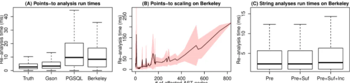
To evaluate the applicability and performance of IncA, we have implemented two Java analyses in IncA adapted from the literature: Strong update points-to analysis [Lhoták and Chung 2011] as well as character-inclusion and prefix-suffix string analysis [Costantini et al. 2011]. Our analyses are intra-procedural, the points-to analysis is flow-sensitive, while the string analyses are flow- insensitive. We ran performance measurements for both analyses on four real-world Java projects with up to 70 KLoC in size. We measured the initial non-incremental run time and the incremental update time after random as well as idiomatic code changes. Our measurements reveal that the initialization takes a few tens of seconds, while an incremental update takes a few milliseconds on average. Additionally, we also benchmarked the memory requirement of the system because incrementalization relies on extensive caching. Our evaluation shows that the memory requirement can grow large but not prohibitive.
In summary, we make the following contributions:
• We identify and describe the key challenge for incremental lattice-based program analysis:
cyclic reinforcement of lattice values (Section 2).
• We present the IncA approach for incremental lattice-based program analysis by embedding in Datalog, requiring recursive aggregation (Section 3).
1https://www.jetbrains.com/mps 2https://github.com/szabta89/IncA
• We develop and verify DRedL, the first algorithm to incrementally solve recursive Datalog rules containing user-defined aggregations (Section 4).
• We implemented DRedLand IncA as open-source software (Section 5).
• We demonstrate the applicability and evaluate the performance of DRedLand IncA on two existing Java analyses (Section 6).
2 CHALLENGES OF INCREMENTAL PROGRAM ANALYSIS
In this section we introduce a running example to illustrate the challenge of incremental lattice-based static program analysis. The example is a flow-sensitive interval analysis for Java, which reports the possible value ranges of program variables. As a starting point, we choose logic programming in Datalog because the use of Datalog for program analysis is well-documented [Green et al. 2013;
Smaragdakis and Bravenboer 2011], and there exist incremental Datalog solvers [Gupta et al. 1993;
Mitschke et al. 2014;Szabó et al. 2016]. It will become clear in this section that incremental program analysis requires incremental recursive aggregation, which existing solvers fail to support.
Interval Analysis with Datalog.A flow-sensitive interval analysis keeps track of the value ranges of variables at each control flow location. We first analyze a program’s control flow by constructing a relationCFlow(src,trg), where each(src,trg)tuple represents an edge of the control flow graph (CFG). We defineCFlow(src,trg)through Datalog rules.
A Datalog rulerhas formh :- a1,...,an wherehis theheadof the rule anda1,...,anare the (possibly negated)subgoals. In standard Datalog (as opposed to some extensions of it [Green et al. 2013]), the rule head and subgoals are of the formR(t1,...,tk)whereRis the name of a relation andti is a term that is either a variable or a constant value. Each rule is interpreted as a universally quantified implication: For each substitution of variables that satisfies all subgoals ai, the headhmust also hold. Given a rule headR(t1,...,tk), the satisfying substitutions of the termst1,...,tkyield the tuples of relationR. We refer the reader to [Green et al. 2013] for further literature on Datalog. The following rules computeCFlow:
CFlow(from, to) :−Next(from, to), ¬IfElseStmt(from).
CFlow(while, start) :−WhileStmt(while), FirstChild(while, start).
CFlow(last, while) :−WhileStmt(while), LastChild(while, last).
First, control flows from a statement to its successor statement if the former is not anIfElseStmt (or any other construct that redirects control flow). Second, control flows from awhilehead to the first child in its body. And third, control flows from the last statement of a loop body to the loop head.Figure 1B shows an example subject program with statementsN1toN5; its CFG as computed byCFlowis shown inFigure 1A.
We now construct a flow-sensitive interval analysis on top of this CFG. We define a relation IntervalAfter(stmt,var,iv), where a tuple(s,v,i)∈IntervalAfterdescribes that after exe- cution of statements, variablevmust take a value in intervali. Termssandvare existing program elements, andiis a computed value from theinterval lattice. To compute the intervaliof variable vafter statements, the analysis must consider two cases. Ifs(re)assignsv, we computev’s interval based on the assignment expression. Otherwisev’s interval does not change, and we propagate the interval associated withvfrom before the statement:
IntervalAfter(stmt, var, iv) :− AssignsNewValue(stmt, var), AssignedInterval(stmt, var, iv).
IntervalAfter(stmt, var, iv) :− ¬AssignsNewValue(stmt, var), IntervalBefore(stmt, var, iv).
In order to figure out this previous interval, we query the CFG to find all control-flow predecessors of the current statement and collect the variable’sIntervalAfterfor each of the predecessors in a relationPredecessorIntervals. As the interval containmentpartial orderforms alattice, we
N3 src
N4 trg
N5 N2
N5
N3 N1
N4
N2
N2 CFlow
iv
[-1,∞) [11,11]
[-1,∞) [11,11]
[-1,∞) [9,9]
[-1,∞) [7,11]
[-1,-1]
[7,7]
iv var
y [0,∞)
x [11,11]
[0,∞) y
x [11,11]
[0,∞) y
[9,9]
x
[0,∞) y
y
x [7,11]
x
[0,0]
[7,7]
(N2) while (read()) { (N3) x = 9;
(N4) x = x + 2;
(N5) y = cond ? y : y + 1; } stmt
(N1) x = 7,y = 0;
IntervalAfter C
Interval relies on the CFlow relation to deduce
control flow
D
ɠ ɡ
B
A
-1
cond ? -1 : 0
ɠ
iv
[-1,∞) [11,11]
[-1,∞) [11,11]
[-1,∞) [9,9]
[-1,∞) [7,11]
[-1,0]
[7,7]
ɡ E
ɢ 0
iv
[0,∞) [11,11]
[0,∞) [11,11]
[0,∞) [9,9]
[0,∞) [7,11]
[0,0]
[7,7]
ɢ
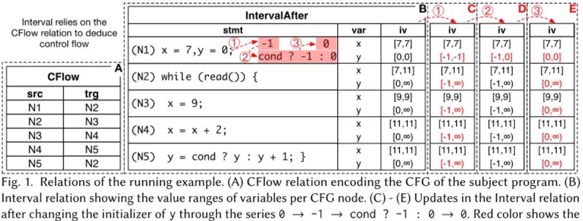
Fig. 1. Relations of the running example. (A) CFlow relation encoding the CFG of the subject program. (B) Interval relation showing the value ranges of variables per CFG node. (C) - (E) Updates in the Interval relation after changing the initializer ofythrough the series0 → -1 → cond ? -1 : 0 → 0. Red color shows the changes compared to previous values.
can obtain the smallest interval containing all predecessor intervals of the current statement. It is computed by aggregating such predecessors using theleast upper bound(lub) lattice operation:
PredecessorIntervals(stmt, var, pred, iv) :− CFlow(pred, stmt), IntervalAfter(pred, var, iv).
IntervalBefore(stmt, var, lub(iv)) :− PredecessorIntervals(stmt, var, _pred, iv).
Note thatIntervalAfter and IntervalBeforearemutually recursive and also induce cyclic tuple dependencieswheneverCFlowis cyclic. This is typical for flow-sensitive program analyses.
We obtain the final analysis result by computing the (least) fixpoint of the Datalog rules. The computation always terminates because the rules in our analysis are monotonic wrt. the partial order of the interval lattice, and because we use widening to ensure that the partial order does not have infinite ascending chains [Cousot and Cousot 2004]. For example, as shown inFigure 1B, the interval analysis computes tuples(N2,x,[7,11])and(N2,y,[0,∞])for the loop head. Tuple (N2,x,[7,11])is the result of joining(N1,x,[7,7])and(N5,x,[11,11]). Tuple(N2,y,[0,∞]) is the result of the fixpoint computation, joining all intermediate intervalslub([0,0], [0,1], [0,2],...)ofybeforeN2.
Incremental Interval Analysis.The analysis presented up to here is standard; we now look at incrementalization. Existing incremental Datalog solvers cannot handle this analysis because they do not support recursive aggregation. The root cause of the limitation is that realistic subject programs typically have loops or recursive data structures. Analyzing them requires fixpoint iteration over cyclic control flow or data-flow graphs, which, in turn, requires recursive aggregation.
Indeed, there is no known algorithm for incrementally updating aggregation results over recursive relations with cyclic tuple dependencies.
The goal of anincrementalanalysis is to update its results in response to the subject program’s evolution over time withminimal computational effort. For illustrative purposes, we consider three changes 1 , 2 , and 3 of the initializer ofyinFigure 1B, and then we review what is expected from an incremental analysis in response to them. First, we change it from0to-1.Figure 1C shows the updatedivcolumn of relationIntervalAfter. While this change does not affect previous results ofx, the intervals assigned toyrequire an update at all CFG nodes. After a subsequent change from-1to(cond ? -1 : 0)we expect that only the interval atN1gets updated (seeFigure 1D) because the analysis of the loop already consideredy=0before. Third, consider a final change from (cond ? -1 : 0)to0. Now the analysis does not have to considery=-1anymore, and we expect an update to all lower bounds of the intervals assigned toyas shown inFigure 1E.
How can we update a previous result with minimal computational effort in response to changes 1 , 2 , and 3 ? Fundamentally, we propagate program changes bottom-up through the analysis’
Datalog rules, starting at the changed program element. For example, a change to a variable’s initializer directly affects the result ofAssignedInterval, which is then used in the first rule of IntervalAfter. If the new initializer has a different interval than the old initializer,AssignedIn- tervalpropagates a derived change toIntervalAfter. A derived change leads to the deletion of the old interval and the insertion of the new interval into the relevant relation. In turn,In- tervalAfterpropagates such a change toPredecessorIntervals, which propagates it to the aggregation inIntervalBefore, which propagates it to the second rule ofIntervalAfter, and so on. This way we can handle change 1 , where we delete(N1,y,[0,0]), insert(N1,y,[-1,-1]), and propagate these changes.
Handling change 2 efficiently is more challenging: We must augment our strategy to avoid deleting(N1,y,[-1,-1])before inserting(N1,y,[-1,0]), so that we can reuse previous results.
Failing to do that would result in re-computing the exact same result, which is unnecessary excess work degrading efficiency.
The toughest problem is change 3 , where we delete(N1,y,[-1,0])and insert(N1,y,[0,0]).
The problem manifests at CFG nodeN2and is due to the loop in the CFG and thelubaggregation over it. Before change 3 ,N2’s CFG predecessorsN1andN5report intervals[-1,0]and[-1,∞)for y, as shown inFigure 1D. When propagating deletion(N1,y,[-1,0])and insertion(N1,y,[0,0]) to N2, we expect to replace (N2,y,[-1,∞)) by(N2,y,[0,∞)). However, the aggregation in IntervalBeforeforN2also has to consider interval[-1,∞)fromN5andlub([0,0], [-1,∞))
= [-1,∞). However, note how this yields thewrongresult forN2because the very reason for [-1,∞) at N5is the old initializer at N1, which just got deleted. We call this situation cyclic reinforcementof lattice values. An incremental analysis must carefully handle cyclic reinforcements to avoid computing incorrect analysis results. The design of an algorithm for executing program analyses incrementally and correctly is the central contribution of this paper.
Problem Statement.Our goal is to incrementalize program analyses with recursive, user-defined aggregations. Our solution must satisfy the following requirements:
Correctness (R1):An incremental analysis must produce the exact same result as re-running the analysis from scratch. For example, it must rule out cyclic reinforcements.
Efficiency (R2): An incremental analysis must update its results with minimal computational effort. We expect from an incremental analysis to be significantly faster than the correspond- ing non-incremental analysis, so that we can use analyses in interactive editing scenarios.
Expressiveness (R3): Our solutions should apply systematically to any program analyses that use (one or more) user-defined lattices and user-defined aggregation operators.
Note that we do not mentionprecisionorrecallbecause these are the responsibility of the analysis developer when designing the lattices and their operations. There is no limitation on the design of those by our solution. However, a more precise analysis might take more time to compute (e.g.
because we reach a fixpoint in more iterations), so it has an impact on performance, just like in a non-incremental analysis.
3 INCREMENTAL LATTICE-BASED PROGRAM ANALYSIS WITH IncA
IncA is a framework for specifying and incrementally executing program analyses that perform recursive lattice-based aggregations. IncA provides a DSL for the specification of lattices and program analyses. As we describe inSection 5, the DSL compiles to Datalog-style rules similar to the ones we have shown inSection 2. In the present section, we focus on the runtime system of IncA and how it executes analyses incrementally.
As pointed out inSection 1, this work extends our prior work on incremental program analysis.
The prior version of IncA could only incrementally analyze relations over program elements; for example, we used it for an incremental points-to analysis for C. However, because of fundamental limitations in the runtime system, there was no support for lattices nor aggregation over them. In this paper, we solve these limitations by adding support for lattice-based aggregations, which, as we have argued above and validate inSection 6, enables a much wider range of program analyses.
3.1 Incremental Execution of Non-Recursive Analyses
The runtime system of IncA incrementally computes relations described by Datalog-style rules. We briefly review program representation, handling of program changes, and non-recursive aggrega- tions first. Then we discuss recursive analyses inSection 3.2.
Program representation and change.We represent the abstract syntax tree (AST) of a program in base relations(extensional predicates in Datalog). We use a separate base relation for each AST node type, for example,IfElseStmtandAssignStmt. We use additional base relations to connect AST nodes, for example,Next(prev,next)for subsequent nodes in a list andParent(child,parent) to represent the containment hierarchy. We rely on the IDE to incrementally maintain the base relations for the subject program, either by incremental parsing [Ramalingam and Reps 1993], non- incremental parsing with tree diffing [Dotzler and Philippsen 2016], or projectional editing [Voelter et al. 2014]; we use the latter.
Program analyses and analysis results.Traditionally, a program analysis traverses the AST of a program to extract analysis results. Correspondingly, in IncA, program analyses query the base relations. That is, program analyses are Datalog-style rules that definederived relations. For example, inSection 2we showed rules that define the derived relationCFlowbased onIfElseStmt, Next, and others. Derived relations can also make use of the contents of other derived relations, which is useful for decomposing an analysis into multiple smaller parts. For example, we defined PredecessorIntervalsbased onCFlow.
IncA allows updates to derived relations to be observed. For example, we can extend our interval analysis to define a derived relationBoundedArrayAccess that contains a tuple for each array access where the interval of the index is guaranteed to be within bounds of the array. By observing this relation, an IDE can incrementally highlight safe and (possibly) unsafe array accesses.
Change propagation.IncA ensures that derived relations are up-to-date; as tuples are inserted and deleted from base relations, IncA propagates these changes to dependent derived relations.
Effectively, IncA maintains a dependency graph between relations and caches their tuples. The base relations are sources of changes, and the IDE-observed derived relations are sinks of changes.
IncA propagates tuples from sources to sinks, and it skips the propagation where a relation is not affected by an incoming change. This can happen in two cases: (i) The cache of the derived relation already accounts for the tuple, or (ii) a Datalog rule ignores the tuple entirely. The first case occurs when the tuple was already derived before through an alternative derivation, which can happen because there can be alternative bodies for the same Datalog rule head. For example, change 2 in Figure 1B was skipped at statementN2because the previous analysis result remained valid. The second case for skipping occurs when an incoming tuple simply could not affect the contents of a relation. For example,booleanvariables are irrelevant for our interval analysis. This manifests in those Datalog rules that inspect the right-hand sides of assignments, but never query relations such asAndExprthat representbooleanexpressions. The IncA compiler optimizes the subject analyses to avoid the propagation of irrelevant changes, see more details in [Szabó et al. 2016].
Finally, the occurrence of negated subgoals in a rule’s body leads to a stratification of change propagation. That is, the relation that occurs negated must be fully up-to-date before we can draw conclusions about the absence of a tuple. For example, in our control-flow analysis, we must fully update relationIfElseStmtbefore we can derive changes toCFlowbased on it. Moreover, when CFlowuses¬IfElseStmt, an insertion intoIfElseStmttriggers deletion(s) fromCFlow, and a deletion fromIfElseStmttriggers insertion(s) intoCFlow. IncA’s change propagation respects negation. Stratification requires that there is no recursion through negation because then we could not fully compute the negated relations before computing the non-negated ones.
Non-recursive aggregation.In contrast to other incremental systems [Gupta and Mumick 1995], IncA supports aggregations overrecursiverelations. Here, however, we first review how IncA handlesnon-recursive aggregations, which, while much simpler, is an important stepping stone.
Formally, an aggregating Datalog rule has the following form:
Agg(t1,...,tk,α(v)) :- Coll(t1,...,tk,_x1,...,_xl,v).
Here theaggregandcolumnvandaggregate resultcolumnα(v)are both lattice-valued, andα is anaggregation operator, i.e. a mapping from amultisetof lattice values to a single lattice value.
Without loss of generality (as shown below) we assume this is the only rule withAggin the head.
We callAggthe aggregating relation andCollthecollectingrelation;t1,. . . ,tkare thegrouping variables, while_x1,. . . ,_xl areauxiliaryvariables.
For example, in the interval analysis fromSection 2,PredecessorIntervalsserved the role of CollwhereasIntervalBeforeserved the role ofAgg, whileα waslub. We usedstmtandvar as grouping variables (the value ofvarafter statementstmt), and we usedpredas an auxiliary variable to enumerate the interval values of all CFG predecessors.
For each substitution of the grouping columns, the aggregand valuesvinColl, if any, are mapped byα into the aggregate result column of the single corresponding tuple inAgg. Given a set of grouping valuest1,...,tk, different sets of values_x1,...,_xl can have the same aggregandv associated with them, soαaggregates over amultisetof values (instead of just a simple set).
Note that the above form of the aggregating rule does not restrict expressiveness (R3): the IncA language actually allows multiple alternative rules forAgg, each with several subgoals. The compiler then introduces a helper relationCollthat is derived using these multiple rule bodies, and then aggregatesAggfromColl.
We can incrementalize non-recursive aggregations by (i) incrementally maintainingCollas usual and (ii) incrementally maintaining the aggregate resultα(v)of each group whenever an aggregand vis inserted or deleted from the collecting relation. IncA specifically supports (seeSection 4.4) the latter kind of incrementality for aggregation operators that are induced by associative and commutative binary operations, e.g.lub(least upper bound) orglb(greatest lower bound).
The above form of aggregating rules is independent of whether the aggregation is recursive or not. An aggregation is recursive ifCollalso depends onAgg(e.g. see dependencies between PredecessorIntervals,IntervalAfter, andIntervalBeforeinSection 2). This leads us to the next part where we discuss recursive analyses.
3.2 Incremental Execution of Recursive Analyses
Our strategy for incrementalizingnon-recursive analyses is relatively simple once the analysis is formulated as a relational computation (e.g., through our DSL,Section 5): We propagate changes through the dependency graph, we are careful about negations, and we incrementally maintain aggregate results. Adding recursion, the process is severely complicated because of cyclic reinforce- ment, as shown inSection 2.
To deal with recursion, we modify our approach in two steps. First, we addrecursive relations but the aggregations must remain non-recursive. This enables the incrementalization of control flow analysis as well as set-based data-flow analyses and represents the current state of the art of incremental Datalog solvers (including the prior version of IncA as documented in [Szabó et al.
2016]). Second, we addrecursive aggregationson values of lattices with monotonic lattice operators.
This enables the incrementalization of lattice-based data-flow analyses and goes beyond the state of the art. We carefully engineer our solution to handle cyclic reinforcement of lattice values correctly, thus satisfyingCorrectness (R1).
Recursive relations.In contrast to non-recursive relations, recursive relations require a fixpoint computation. That is, an insertion into a recursive relation can trigger subsequent insertions, which can trigger subsequent insertions, and so on. Consider the following recursive relation that computes the transitive closure ofCFlow:
CFlowReach(from, to) :−CFlow(from, to).
CFlowReach(from, to) :−CFlow(from, step), CFlowReach(step, to).
When adding a statementstmtto the program, we trigger an insertion of (pred,stmt)into CFlowforstmt’s predecessor. This triggers subsequent insertions such as(predpred,stmt)into CFlowReachforpred’s predecessor, but eventuallyCFlowReachstabilizes when no new tuples can be derived.
Incrementally deleting tuples from a recursive relation is more difficult because of cyclic rein- forcement of tuples. If a tuple was derived multiple times within a cycle, deleting one derivation does not necessarily invalidate the other derivations, but invalidating all derivations is sometimes necessary to obtain correct results. This is similar to the cyclic reinforcement of lattice values we discussed inSection 2, with an important difference: The cyclic reinforcement of tuples does not involve aggregations.
There is a generic solution called Delete and Re-derive (DRed) [Gupta et al. 1993] for supporting deletions in spite of cyclic reinforcement of tuples. The basic strategy of DRed is to first delete the tuple and everything that was derived from it, ignoring alternative derivations of that tuple for now. This is an over-approximation and, in general, will delete too much. After the deletion reaches a fixpoint, DRed starts a re-derive phase to insert back all those tuples that can be derived from the remaining ones that were left intact during the delete phase.
Recursive aggregation.The key technical contribution of our paper is to develop a novel algorithm for incremental recursive aggregation in Datalog. As we explained inSection 2, the main challenge is the cyclic reinforcement of lattice values (in contrast to cyclic reinforcement oftuples, as discussed above). Specifically, change 3 inFigure 1B induced the deletion of tuple(N1,y,[-1,0]), which should have triggered the deletion of(N2,y,[-1,∞)). However, becauseN2occurred in a loop, there was cyclic reinforcement between the lattice values:N5still reported the interval[-1,∞), even though the very reason for that value is that the initial interval was[-1,0]previously. At this point, we did not know how to proceed.
Why can we not just apply DRed here? How is cyclic reinforcement of lattice values different from cyclic reinforcement of tuples? The main difference is that updating an aggregate value induces both a deletion of the old value and an insertion of the new value. However, DRed first processes all deletions and postpones insertions until the re-derive phase. Hence, one issue is that lattice values require an interleaving of the delete and re-derive phases, which violates the contract of DRed. A second issue is more subtle. Let’s say we allow interleaving. When deleting the old aggregate value, DRed’s delete phase will delete all tuples derived from it. In particular, it will delete the new aggregate value, which we were just about to insert.
To resolve these issues, we developed a novel algorithm called DRedL. It generalizes DRed to support incremental computation of recursivemonotonicaggregations over lattices. Given a partially ordered set(M,⊑), an aggregation operatorαis⊑-monotonic ifα(M) ⊑ α(M ∪ {m})
⊑ α(M ∪ {m’})for all multisets of valuesM ⊆ Mand all valuesm,m’ ∈ Mwithm⊑m’. That is, the aggregate result of a monotonic aggregation increases with the insertion of any new tuple or with the increasing replacement of any existing tuple in the collecting relation.
Crucially, our algorithm recognizes monotonicity at runtime when handling the update of an aggregate result. Given a⊑-monotonic aggregatorα, whenever DRedLsees a deletion(t1,..., tk,old)from a relation and an insertion(t1,..., tk,new)to the same relation withold ⊑ new, it recognizes that together they represent an increasing replacement of a lattice value. We call such a change pair a⊑-increasing replacement, and deletions that are part of a⊑-increasing replacement do not need to go through a full delete phase. This way, deletions of old aggregate results will not invalidate cyclically dependent lattice values and, in particular, the new aggregate values. This allows DRedLto perform correct incremental maintenance even in presence of recursive aggregation.
We describe the details of DRedLinSection 4, with a focus on correctness and efficiency; its novelty over the state-of-the-art (esp. DRed) will be discussed inSection 7.
While inSection 4we explain DRedLin its full generality, its main application is the incremen- talization of program analyses that use custom lattices. Program analyses routinely use lattices to approximate program behavior [Nielson et al. 2010]. Without recursive aggregation, only the power set lattice can be represented because recursive tuple insertion and deletion can model set union and intersection. DRedL’s support for recursive aggregation lifts this limitation and enables the incrementalization of program analyses over any user-defined lattice. InSection 6, we show how DRedLperforms on strong-update points-to [Lhoták and Chung 2011] and string analyses [Costantini et al. 2011].
4 INCREMENTAL RECURSIVE AGGREGATION WITH DREDL
We design DRedL, an incremental algorithm for solving Datalog rules that use recursive aggregation over lattices. Given a set of Datalog rules, DRedLefficiently and transitively updates derived relations upon changes to base relations.
DRedLpropagates changes to derived relations in the four steps described below, which are similar to earlier algorithms (notably DRed). However, there are key differences at each step, necessitated by the support for lattice aggregation, that will be discussed inSection 7.
(1)Change splitting: Split incoming changes into monotonic changes (increasing replacements and insertions) and anti-monotonic changes (deletions that are not part of increasing replace- ments). The crucial novelty over the older DRed algorithm is the lattice-aware recognition of increasing replacements at runtime, which heavily impacts the other three steps as well.
(2)Anti-monotonic phase: Interleaved with the previous step, we process anti-monotonic changes by transitively deleting the relevant tuples and everything derived from them. This is an over-approximation and, in general, will delete too much, but, importantly, over-deletions guarantee that we compute correct results in the face of cyclic reinforcements.
(3)Re-derivation: Fix the over-approximation of the previous step by re-deriving deleted tuples from the remaining tuples.
(4)Monotonic phase:Process monotonic changes. For insertions, we insert the new tuple and transitively propagate the effects. For increasing replacements, we simultaneously delete the old tuple and insert the new tuple and transitively propagate their effects. By propagating deletions and insertions of increasing replacements together, we ensure that dependent relations will in turn recognize them as increasing replacements and handle them accordingly.
In the remainder of this section, we summarize the assumptions of DRedL on Datalog rules, introduce necessary data structures for DRedL, present DRedLas pseudocode, explain how DRedL
incrementalizes aggregations, and present a proof sketch of our algorithm.
4.1 Assumptions of DRedLon the Input Datalog Rules
In order to guarantee that DRedLcomputes a correct (R1) analysis result efficiently (R2), the input Datalog rules must meet the following assumptions:
Monotonic recursion (A1): We call a set of mutually recursive Datalog rules adependency component. DRedLassumes that each dependency component respects a partial order⊑of each used lattice (either the natural order of the lattice, or its inverse). Given this order, the relations represented by the rules must only recur⊑-monotonically: If they are updated by insertions or⊑-increasing replacements, thenrecursivelyderived results may only change by insertions or⊑-increasing replacements. This assumption has important implications:
Abstract interpretation operators and aggregations must be monotonic within a dependency component wrt. the chosen partial order. The analysis developer needs to ensure operators are monotonic. Additionally, recursion through negation is not allowed: IncA automatically rejects analyses that do not conform to this requirement (Section 5).
Aggregation exclusivity (A2) Alternative rules deriving the same (collecting) relation must produce mutually disjoint results, if the relation is in a dependency component that uses aggregation at all. This is important for ruling out cyclic reinforcements.
Cost consistency (A3)Given a non-aggregating relationR(t1,...,tk,v)with lattice-typed columnv, we require that columns(t1,...,tk)uniquely determine columnv.
No infinite ascending chains (A4)DRedLcomputes the least fixpoint of the Datalog rules.
To ensure termination and as is standard in program analysis frameworks, DRedLrequires that the used lattices do not contain infinite⊑-ascending chains [Atiyah and Macdonald 1994, Section 6] for any ⊑ that is chosen as part ofA1. Fulfilling this requirement may require widening [Cousot and Cousot 2004], as shown in our interval analysis inSection 2.
AssumptionA1allows a dependency component to use and aggregate over several lattices. For each of those, the component must be monotonic; this is the responsibility of the analysis developer.
In many typical lattice analyses (e.g. where aggregators are idempotent likelub,glb), the IncA compiler can automatically guaranteeA3by transforming the IncA analysis code (using the idea in [Ross and Sagiv 1992] as detailed inSection 5.3). In other cases, it is the responsibility of the analysis developer. For non-aggregating standard Datalog programsA2trivially holds.
We validated that these assumptions suffice for correctness (R1) by constructing a proof sketch (Section 4.5). We also validated that these assumptions do not inhibit expressiveness (R3) for incremental program analyses by construction of IncA (Section 5) and case studies (Section 6).
4.2 Support Data Structures
The anti-monotonic step of DRedLperforms an over-deletion, after which some tuples may need to be re-derived; while the monotonic phase performs monotonic deletions that do not always have to be propagated. To make these decisions, we adapt support counts [Gupta et al. 1993] for tuples, and we design a new data structure called support multisets for aggregate results:
• Support count: The support count of a tuple is equal to the number of alternative derivations a tuple has within a relation (across all alternative rules and local variables). Given a tuplet in relationR,Support#R(t)represents the support count oft.
• Support multiset: The support multiset of an aggregate result contains the individual aggre- gands that contribute to it. Formally, given an aggregating rule as inSection 3.1, the support
procedure maintainIncrementally(all) { 1
for C in top. order of dep. components { 2
effect:= immediateConsequences(C, all) 3
(anti,mon):= changeSplitting(effect) 4
deleted:= ∅ 5
while (anti != ∅) {//ANTI-MONO - fixpoint 6
new:= updateAnti(anti);deleted ∪= new 7
newEffect:= immediateConsequences(C, new) 8
(anti,mon):=changeSplitting(newEffect∪mon) 9
} 10
red:= directRederive(deleted) // RE-DERIVE 11
mon ∪= immediateConsequences(C, red) 12
all ∪= deleted ∪ red 13
while (mon != ∅) { //MONO - fixpoint 14
new:= updateMon(mon); all ∪= new 15
mon:= immediateConsequences(C, new) 16
}}} 17
procedure directRederive(deleted) { 36
red:= ∅ 37
foreach change in deleted { 38
R:= rel(change) 39
if (R is non-aggregating) { 40
if (Support#R(|change|) > 0) 41
red ∪= { +|change| } 42
} else { // aggregating: R(t,α(v)):-... 43
let R(t,v) = |change| 44
if (SupportMSR (t) != ∅) { 45
red ∪= { +R(t,α(SupportMSR (t))) } 46
} 47
} 48
} 49
update stored relation contents by red 50
return red 51
} 52
procedure updateAnti(body) { 18
head:= ∅ 19
foreach change in body { 20
R:= rel(change); h:= πR(change) 21
if (R is non-aggregating) { 22
Support#R(|h|) -= 1 23
if (|h| ∈R) 24
head ∪= {h} 25
} else { // aggregating: R(t,α(v)) 26
let R(t, v) = |h| 27
SupportMSR (t) -= {v} 28
if (∃w. (t, w) ∈ R) 29
head ∪= {−R(t, w)} 30
} 31
} 32
update stored relation contents by head 33
return head 34
} 35
procedure updateMon(body) { 53
head:= ∅ 54
foreach change in body { 55
R:= rel(change); h := πR(change) 56
if (R is non-aggregating) { 57
Support#R(|h|) += sign(h) 58
if (support changed to or from 0) 59
head ∪= {h} 60
} else { // aggregating: R(t,α(v)) 61
let R(t, v) = |h| 62
head ∪= {-R(t,α(SupportMSR (t)))} 63
if (sign(h) == -1) { SupportMSR (t) -= {v} } 64
else { SupportMSR (t) += {v} } 65
head ∪= {+R(t,α(SupportMSR (t)))} 66
}} 67
update stored relation contents by head 68
return head 69
} 70
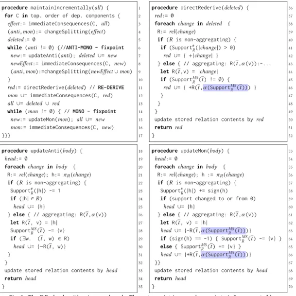
Fig. 2. The DRedLalgorithm in pseudocode. The entry point is procedure. maintainIncrementally.
multiset SupportMSAggassociates, to each substitution of grouping variables of aggregating rela- tionAgg, the aggregands in the group fromColl. In other words,SupportMSAgg(t1,...,tk)is the multiset of valuesvthat satisfyColl(t1,...,tk,_x1,...,_xl,v)for some_x1,...,_xl. These support data structures are used and incrementally maintained throughout DRedL. As Support#Ris no larger thanRand SupportMSAggis no larger thanColl, there is no asymptotic overhead.
4.3 DRedLAlgorithm
We present the DRedLalgorithm as pseudocode inFigure 2. The entry point is proceduremain- tainIncrementally, which takes a changesetallas input and updates affected relations. In the code, we use italic font exclusively for variables that store changesets.
As usual for incremental Datalog solvers, DRedLiterates over the dependency components of the analysis in a topological order (Line 2). We exploit that recursive changes within each component
are required to be monotonic (AssumptionA1). We start in Line 3 by computing theimmediate consequencesof changes inallon the bodies of the Datalog rules in the current componentC.
That is, for a Datalog ruleh :- a1,...,an inC, we compute the consequences of the changes on a1,...,anfirst. We omit the details ofimmediateConsequences, but the implementation relies on straightforwardalgebraic differencingfrom the Datalog literature [Gupta and Mumick 1995].
Technically, the interim resulteffectis expressed on rule bodies and not yet projected to rule heads likeh(the actual relations to be maintained). This allows us to maintain support counts and support multisets for alternative body derivations.
If componentCuses aggregation, in Line 4 we performchange splittingof changeseteffect, according to the⊑of AssumptionA1. We compute the set ofmonotonic changes monfromeffect by collecting all insertions and those deletions that are part of an increasing replacement:
mon = {+r(t1, . . . ,tk) | +r(t1, . . . ,tk)∈effect}
∪ {−r(t1, . . . ,tk,cold)| −r(t1, . . . ,tk,cold)∈effect,+r(t1, . . . ,tk,cnew)∈effect,cold ⊑cnew} Here and below we write+r(t1, . . . ,tk)for a tuple insertion and−r(t1, . . . ,tk)for a deletion. The set ofanti-monotonic changesconsists of all deletions not inmon. Note that for a componentCthat does not use aggregation,monsimply consists of all insertions andanticonsists of all deletions.
Next, we perform theanti-monotonic phaseon changesetantiiteratively until reaching a fixpoint (Line 6-10). In each iteration, we first use procedureupdateAnti(discussed below) to update the affected support data structures and relations (Line 7). This yields changesnewto rule heads defined inC. We propagate thenewchanges todeletedbecause they are candidates for a later re-derivation. But we also propagate thenewchanges toCto handle recursive effects (Line 8), yielding recursive feedback innewEffect. By design, the anti-monotonic phase within a dependency component only produces further deletions and never insertions. We merge thenewEffectchanges with the monotonic changesmonand split them again because a new change may cancel out an insertion or form an increasing replacement. Note that this can be done efficiently by indexing the changesets for aggregating relations over the grouping variables. This way we can efficiently query relevant lattice values when deciding if a pair needs to be split up or formed.
ProcedureupdateAntiprocesses anti-monotonic changes of rule bodies and projects them to changes of the rule heads while keeping support counts and support mutlisets up-to-date. We iterate over the anti-monotonic body changes, all of which are deletions by definition. For each change, we obtain the changed relation symbolR, and we project withπRthe body change to the corresponding change of the relation’s headh(Line 21). Whilehis a change, we write|h|to obtain the change’s absolute value, that is, the tuple being deleted or inserted. IfRdoes not aggregate, we decrease the support count ofhand we propagate a deletion ofhif it is currently derivable inR.
If insteadRaggregates, we decomposehto obtain the grouping termstand the aggregandv. We deletevfrom the support multiset oft. Furthermore, ifRcurrently associates an aggregation result wtot, we propagate the deletion of said association fromR. Note that the associated aggregation resultwis unique by AssumptionA3, and we delete it as soon as any of the aggregands is deleted. It is important to point out that a positive support count or non-empty support multiset after deletions is no evidence for the tuple being present in the relation, due to the possibility of a to-be-deleted tuple falsely reinforcing itself through cyclic dependencies. We will put back tuples that still have valid alternative derivations, and we will put back aggregate results computable from remaining aggregands in the re-derivation step of DRedL. Finally, we update the stored relations and return headfor recursive propagation in the main proceduremaintainIncrementally.
Back inmaintainIncrementally, we proceed withre-derivationto fix the over-deletion from the anti-monotonic phase (Line 11-12). To this end, we use proceduredirectRederiveto re-derive tuples that were deleted during the anti-monotonic phase but still have support. The input to the
procedure isdeleted, and we iterate over the deletions in the changeset. IfRdoes not aggregate, we use the support count: A positive support count indicates the tuple is still derivable, and we propagate a re-insertion (Line 41-42). If insteadR aggregates, we use the support multiset: A non-empty support multiset indicates that some aggregand values are left (Line 45). In this case, we recompute the aggregation result by applying the aggregation operatorαand propagating a re-insertion (Line 46). Due to the support multiset, we do not need to re-collect aggregand values, saving precious time. InSection 4.4, we explain how we further incrementalize the aggregation computation (blue highlighting in the code). We return to proceduremaintainIncrementallyby storing the re-derived tuples inred. Because these tuples, together with the previously deleted ones, can trigger transitive changes in downstream dependency components, we adddeletedand montoall(Line 13). We perform a signed union, so ultimately if a tuple was deleted but then we could re-derive it, then that tuple will not changeall. Note that re-derivation triggers insertions only and hence only entails monotonic changes that we handle in the final step of DRedL.
Finally, DRedL runs themonotonic phaseuntil a fixpoint is reached (Line 14-16). In each iteration, we use procedureupdateMonto compute the effect of the monotonic changes. Procedure updateMonis similar toupdateAnti, butupdateMonhandles deletions as well as insertions due to increasing replacements. IfRdoes not aggregate (Line 57-60), we update the support count of haccording to the tuple being an insertion (sign(h)=1) or a deletion (sign(h)=-1). If insteadR aggregates (Line 61-66), we delete the old aggregate result and insert the new one. To this end, we compute the aggregate result over the support multiset before and after the change to the support multiset. We collect all tuple deltas and return them tomaintainIncrementally, which continues with the next fixpoint iteration. The implementation also checks if the produced tuple deltas may cancel each other out, which is quite common with idempotent aggregation functions such aslub.
ProceduremaintainIncrementallyexecutes the four steps of DRedL for each dependency componentCuntil all of them are up-to-date. While it may seem that a change requires excessive work, in practice many changes have a sparse effect and only trigger relatively little subsequent changes. We evaluate the performance of DRedLin detail inSection 6. One potential source of inefficiency in DRedLis computing the aggregation result over the support multiset (highlighted in blue inFigure 2). We eliminate this inefficiency through further incrementalization.
4.4 Incremental Aggregator Function
ProceduresupdateAntiandupdateMonrecompute the aggregate results based on support multisets.
A straightforward implementation, that reapplies aggregation operatorαon the multiset contents, will requireO(N)steps to recompute the aggregate result from a multiset ofNvalues. For example, a flow-insensitive interval analysis on a large subject program may write to the same variableN times. For largeN, this can degrade incremental performance as computational effort will linearly depend on input sizeN (instead of the change size), which contradictsEfficiency (R2).
Given associative and commutative aggregation operators (likeglb orlub), our idea is to incrementalize the aggregator functions themselves using the following approach. Independently from the partial order of the lattice we aggregate over, we take an arbitrarytotalorder of the lattice values (e.g., the order of memory addresses). Using this order, we build a balanced search tree (e.g. AVL [Sedgewick and Wayne 2011, Chapter 3.3]) from the aggregands. At each node, we store additionally the aggregate result of all aggregands at or below that node. The final aggregate result is available at the root node. Upon insertion or deletion, we proceed with the usual search tree manipulation. Then we locally recompute the aggregate results of affected nodes and their ancestors in the tree. At each node along the path of lengthO(loдN), the re-computation consist of aggregating inO(1)time the locally stored aggregand with intermediate results. In sum, this way we can incrementally update aggregate results inO(loдN)steps, while usingO(N)memory.
4.5 DRedLSemantics and Correctness Proof
Our approach relies on the formal semantics of recursive monotonic aggregation given byRoss and Sagiv[Ross and Sagiv 1992]. We recap here the most important semantical aspects (taken from [Ross and Sagiv 1992]), and then present a novel proof sketch for the correctness of DRedL. 4.5.1 Semantics of Recursive Aggregation.Adatabaseorinterpretationassigns actual instance rela- tions to the relation names (predicates) appearing in the Datalog rules. A database iscost consistent if it satisfies the condition in AssumptionA3, i.e. lattice columns are functionally determined by non-lattice columns in all relations. Let the set of variables that appear in the body (in any of the subgoals) of a Datalog rulerbeV ars. Then, given a concrete database, one can evaluate the body of a ruler to find all substitutions toV arsthat satisfy all subgoals in the body.
Amodelis a cost-consistent database that satisfies all Datalog rules, i.e. any given derived relation is perfectly reproduced by collecting or aggregating the derivations of all those rules that have this relation in the head. ADatalog semanticsassigns a unique model to a set of Datalog rules (where, technically, base relations are also encoded as rules that only use constants, so calledextensional rules). In the following, we present the semantics ofRoss and Sagivby induction on dependency components, i.e. when considering the relations defined by a given component, we assume that we already know the semantics of all other components it depends on, so they can be equivalently substituted by constants and considered as base relations.
For such a single dependency component, by AssumptionA1we have a partial order⊑for each lattice used. We can thus lift this notation to define a partial order (shown to be a lattice as well) on databases; we say thatD1⊑D2iff for each tuplet1 ∈D1, there is a tuplet2 ∈D2in the corresponding relation such thatt1⊑t2. For cost-consistent databases, this is equivalent to saying D2can be reached fromD1by tuple insertions and⊑-increasing replacements.
It has been shown [Ross and Sagiv 1992] that if a set of Datalog rules satisfy AssumptionA1 andA3, then there is a uniqueminimal modelMmin, i.e. all modelsMhaveMmin⊑M. Thus the minimal model is considered as the semantics of the Datalog rules with recursive aggregation.
4.5.2 Correctness of the Algorithm - Proof Sketch.Following [Green et al. 2013;Motik et al. 2015;
Ross and Sagiv 1992], we give an informal sketch to prove the proposed DRedLalgorithm correct (R1), given the assumptions3fromSection 4.1. We do not include proofs for the correctness of well-known techniques used, such as algebraic differencing [Gupta and Mumick 1995] or semi-naïve evaluation [Green et al. 2013].
Specifically, we will show that DRedLterminates and produces the minimal model, while keeping its support data structures consistent, as well. As usual, we will conduct the proof using (i) induction by update history, i.e. we assume that DRedLcorrectly computed the results before given input changes were applied, and now it merely has to maintain its output and support data structures in face of the change; as well as (ii) componentwise induction, i.e. we assume that the result for all lower dependency components have already been correctly computed (incrementally maintained), and we consider them base relations.
Preliminaries.LetBoldbe the base relations (input) before a changeset∆, inducing minimal model Mminold, which DRedLcorrectly computed by the induction hypothesis; letB=Bold∪∆be the new input andMminthe new minimal model, which DRedLshall compute. LetD∩be the⊑-greatest lower bound of the two minimal models (exists since databases themselves form a lattice [Ross and Sagiv 1992]); essentially it is the effect of applying the anti-monotonic changes only.
3To prove general fixpoint convergence,Ross and Sagivrequired each lattice to be acomplete lattice. We have dropped this assumption in favor of AssumptionA4, which will also suffice for our goals. Note that we require the finite height of ascendingchains only, thus strictly speaking our assumption is neither stronger nor weaker than the original one.
Let we denote byDinit =D0antithe current database (state of base and derived relations) when DRedLstarts to process the dependency component (with changes in base relations already applied), byDiantiafter iterationiof the anti-monotonic phase, byDfinalanti at the end of the anti-monotonic phase, byDred=D0monafter the immediate re-derivations, byDimonafter iterationiof the monotonic phase, and finally byDfinalmon after the monotonic phase.
Monotonicity.Iterations of the anti-monotonic phase only delete tuples, soDinit ⊒Dianti ⊒Dfinalanti. Re-derivations are always insertions, and each re-derived tupletredcompensates for a tupletanti ⊒ tred(tanti =tredfor non-aggregating relations) that was deleted during the anti-monotonic phase;
therefore we also haveDfinalanti ⊑Dred⊑Dinit. Finally, by induction oniand by AssumptionA1, each iterationiof the monotonic phase performs monotonic changes, thusDred ⊑Dimon⊑Dfinalmon.
Termination.The anti-monotonic phase must terminate in finite time as there are finite number of tuples to delete. The immediate re-derivation affects at most as many tuples as the anti-monotonic phase, thus it terminates. The monotonic phase must reach its convergence limit in a finite number of steps as well, for the following reasons. Given a finite database of base relations, a finite amount of non-lattice values are available. Due to AssumptionA3it follows that the output of the component is also finite. As the monotonic phase never deletes tuples, it can only perform a finite number of insertions to reach this finite output size. Finally, it may only perform a finite number of⊑-increasing replacements due to AssumptionA4.
Upper bound and support consistency.We now show that after the anti-monotonic phase, interme- diate database states are upper bounded by the desired output, and that support data structures are consistent: A tupletis (i) contained in the database or (ii) has a positive support count or nonempty support multiset only if∃t′∈Mminwitht⊑t′.
The anti-monotonic phase deleted all tuples that, in any way, depended transitively on the anti-monotonic part of input deletions, therefore those that remained must have had support not impacted by the deletions, thusDantifinal⊑D∩ ⊑Mmin. As rules are monotonic by AssumptionA1, and the support data structures are correctly maintained (using algebraic differencing [Gupta and Mumick 1995] byimmediateConsequences), any tupletthat has support in stateDantifinalmust have at′that has support in (and thus contained in)Mmin. This means that re-derivation only inserts tuples upper bounded by the minimal model, soDred⊑Mmin.
A similar argument applies during the monotonic phase. Assume by induction thatDimon−1 ⊑ Mmin. All tuplest that are to be inserted in iterationi due to having support (as computed by immediateConsequencesand reflected in the support data structures byupdateMon), must have (by AssumptionA1and the induction hypothesis) a correspondingt′ ∈ Mminwitht ⊑t′, thus Dimon⊑Mminstill holds. Eventually,Df inalmon ⊑Mmin.
Cost consistency.We will show that the outputDf inalmon is cost consistent. Base relations are considered cost consistent due to AssumptionA3and the assumed correctness of DRedLfor lower dependency components. Therefore it is sufficient to check the cost consistency of derived relations, which we do by indirect proof. By the induction hypothesis, the state of the algorithm before the change was the cost-consistent modelMminold. The change in base relations did not directly affect derived relations and the anti-monotonic phase only deleted tuples, soDfinalanti is cost-consistent as well. During the re-derive and monotonic phase, tuples are only inserted if they have support, so cost-consistency is only violated if tuplest ,t′, agreeing on all non-lattice columns, both had support. Let us assume such a situation arises, and we prove that it can actually never happen.