Novel Methods for Removing EEG Artifacts and Calculating Dynamic Brain Connectivity
A Thesis Submitted for the Degree of Doctor of Philosophy in Computer Science
Mohamed Fawzy Ibrahim Issa
Supervisors:
Prof. Kozmann György Dr. Juhász Zoltán
Department of Electrical Engineering and Information Systems Doctoral School of Information Science and Technology
University of Pannonia Veszprém, Hungary
2020
DOI:10.18136/PE.2020.753
I
Novel Methods for Removing EEG Artifacts and Calculating Dynamic Brain Connectivity
Thesis for obtaining a PhD degree in
the Doctoral School of Information Science and Technology of the University of Pannonia.
Written by:
Mohamed Fawzy Ibrahim Issa
Supervisors:
Prof. Kozmann György propose acceptance (yes / no) ……….….……..
(supervisor/s)
Dr. Juhász Zoltán propose acceptance (yes / no) ……….….……..
(supervisor/s)
The candidate has achieved 100 % in the comprehensive exam held on 31 May 2018
...
(Head of the Doctoral School) As reviewer, I propose acceptance of the thesis:
Name of reviewer: Prof. Jobbágy Ákos ( yes / no)
...
(reviewer) As reviewer, I propose acceptance of the thesis:
Name of reviewer: Prof. Benyó Balázs ( yes / no)
...
(reviewer) The PhD-candidate has achieved…………. % at the public discussion,
Veszprem, Date:
...
(Chairman of the Committee) Th grade of the PhD diploma ...%
Veszprem, Date:
...
(Chairman of UDHC)
I
Acknowledgment
First and foremost, I would like to express my thanks to ALLAH for guiding and aiding me to bring this work out to light. My deep thanks and highest gratitude go to my supervisors, Prof.
Kozmann György and Dr. Juhász Zoltán for their patience, motivation, enthusiasm, and immense knowledge. I cannot possibly express anymore of my gratitude to them, not only on the guidance they gave during my study as a PhD student but valuable life experiences as well.
I would like to thank the Director of the Doctoral School Prof. Katalin Hangos for her help and support during the doctoral school report presentation. Thanks to the staff of University of Pannonia, especially Ujvári Orsolya, Lényi Szilvia, Dulai Tibor and Görbe Péter. They assisted me in every possible way and went through all the office works for me to have a good experience in Hungary. I would also like to take this opportunity to thank my great friend Dr Tuboly Gergely and his family for his kindness during my accommodation in Hungary.
I acknowledge and thank the Dean and Deputy Dean of the Faculty of Information Technology, Prof. Hartung Ferenc and Dr. Werner Ágnes, for the financial support under the project EFOP- 3.6.1-16-2016-00015. Many thanks to Prof. Zoltan Nagy for giving me access to stroke patient measurements.
My deep thanks to the Egyptian Ministry of Higher Education and Scientific Research and to the Hungarian Ministry of Higher Education for their cooperation with Egypt to have my study in Hungary.
Last but not the least; I would like to thank my family, my parents, whose love and guidance are with me in whatever I pursue. They are the ultimate role models. Most importantly, I wish to thank my loving and supportive wife, Olfat, and my lovely daughter Rokaya who provide unending inspiration.
Mohamed F. Issa, 2020
II
Abstract
Electroencephalography (EEG) is one of the most frequent tools used for brain activity analysis.
Its high temporal resolution allows us to study the brain at rest or during task execution with details not available in traditional imaging modalities. The low cost and simple mode of application enable EEG to be used for studying patient populations to help in the diagnosis and treatment of various brain injuries and disorders such as stroke, Alzheimer’s or Parkinson’s disease.
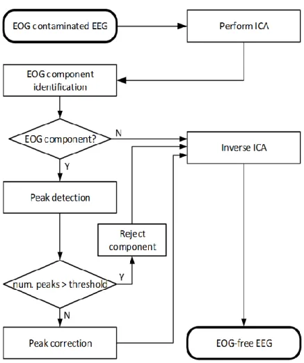
Unfortunately, EEG signals are frequently contaminated by undesirable noise and physiological artifacts, which may distort the underlying true neural information and lead to false diagnoses or unreliable experimental data that cannot be used for valid scientific studies. Consequently, artefact removal is a key step in EEG signal processing, and due to the complexity of the problem, it is still an active, open research area. This thesis presents novel methods developed to solve problems in EEG artifact removal. The fully automatic methods allow us to remove eye movement, blink (EOG) and heart-related (ECG) artifacts without using additional reference channels. Independent Component Analysis (ICA) was applied to the measured data, and the Independent Components (ICs) were examined for the presence of both ECG and EOG. An adaptive threshold based QRS detection algorithm was applied to the ICs to identify ECG activity using a rule-based classifier. EOG artifacts were removed from ocular artifact ICs in a selective way using wavelet decomposition minimising the loss of neural information content during the artifact removal process.
The second part of the thesis focuses on functional connectivity methods that allow the construction of resting state and task-related brain activity networks. First, resting state connectivity methods were used to analyse stroke patient brain activity in order to discover potential biomarkers for stroke recovery. Data set was recorded form healthy volunteers and stroke patients during resting state and functional connectivity graphs were created for the delta, theta, alpha and beta frequency bands. A comparison was performed between patients and control subjects as well as between start and end of the stroke rehabilitation period. The results showed differences in the graph degree, clustering coefficient, global and local efficiency that correlate with brain plasticity changes during stroke recovery, and that these can be used as biomarkers to identify stroke severity and outcome of recovery.
To uncover changes in the connectivity network during task execution, Dynamic Brain Connectivity (DBC) methods must be used. Traditional techniques to reveal temporal changes are based on the Short-Time Fourier Transform or wavelet transformation, which have limits on temporal resolution due to the time-frequency localization trade-off. In this work, a high time- frequency resolution method using Ensemble Empirical Mode Decomposition was proposed that generates phase-based dynamic connectivity networks based on the instantaneous frequency of the signals. A comparison with sliding-window techniques was conducted to validate the accuracy of the method. The results showed that the new method can track fast changes in brain connectivity at a rate equal to the sampling frequency.
III
Összefoglaló
Az EEG (elektroenkefalográfia) az egyik leggyakrabban használt eszköz az agy aktivitásának vizsgálatára. Nagy időbeli felbontásának köszönhetően lehetővé teszi az agy nyugalmi és feladat- végrehajtás közbeni működésének olyan részletességű vizsgálatát, ami más képalkotó módszerekkel nem lehetséges. Alacsony költsége és egyszerű alkalmazhatósága miatt nagy jelentősége van különböző idegrendszeri betegségek és agysérülések (sztrók, epilepszia, Alzheimer és Parkinson betegség) diagnosztikájában és kezelésében.
Sajnos az EEG mérési jelek gyakran tartalmaznak nemkívánatos zajokat és műtermékeket, amik eltorzíthatják az eredeti idegi működésre jellemző információt és így hamis diagnózist adhatnak, vagy az adat annyira megbízhatatlan lehet, hogy az alkalmatlan tudományos vizsgálatokra.
Emiatt a zaj- és műtermék-mentesítés egy fontos lépés az EEG jelfeldolgozás során. A probléma komplexitása miatt ez jelenleg is aktív kutatási terület. Ez a disszertáció új műtermék eltávolítási módszereket ismertet, amik a jelenleg ismerteknél jobb eredményeket nyújtanak. A teljesen automatikus eljárások lehetővé teszik a szemmozgások, pislogás és a szívműködés okozta műtermékek eltávolítását a megszokott extra referencia elektródák (EOG, EKG) használata nélkül. Független komponens analízist alkalmazva, a mért adatok független komponensekre bontása után, a szemmozgás és EKG műtermékeket reprezentáló komponenseket azonosítom és eltávolítom. Az EOG műtermék komponens esetén nem a teljes komponenst távolítom el a jelből, hanem wavelet dekompozíciót alkalmazva, szelektíven tisztítom meg a szemmozgás műtermékektől, így minimalizálva a jelben található neurális információ minimális torzulását.
A disszertáció második része a funkcionális konnektivitási módszerekre fókuszál, melyek lehetővé teszik az agyi nyugalmi hálózatok, illetve a feladat végrehajtás közben kialakuló hálózatok feltérképezését. Elsőként a nyugalmi hálózatok létrehozására alkalmas módszereket vizsgáltam meg a sztrók rehabilitációt elősegítő biomarkerek azonosítása céljából. Egészséges és beteg EEG adatok felhasználásával konnektivitási hálózatokat készítettem a delta, théta, alfa és béta frekvencia sávokban. A sztrók beteg nyugalmi hálózatait összehasonlítottam a kontrol személyekével és megvizsgáltam a különbséget a sztrók bekövetkezése után egy héttel és három hónappal. Az eredmények azt mutatják, hogy a konnektivitási gráf fokszáma, a klaszterezési együttható, a globális és lokális hatékonyság korrelál a sztrók alatt lezajló agyi plaszticitás mértékével, és felhasználható biomarkerként a sztrók súlyosságának és a javulás mértékének előrejelzése céljából.
A feladat-végrehajtás agyi mechanizmusainak pontosabb megértését segítheti a dinamikus funkcionális konnektivitás (DBC) módszer alkalmazása. A hagyományos módszerek, melyek a konnektivitási gráf időbeli változásait határozzák meg, általában a rövid idejű Fourier transzformációra (STFT) alapulnak. Ezeknek a pontosságát behatárolja az idő-frekvencia felbontás határozatlansági tulajdonsága. A dolgozatban egy olyan új, nagy időbeli felbontást eredményező módszert fejlesztettem ki, ami az empirikus dekompozícióra alapulva, a jelek azonnali fázis információját képes meghatározni, amiből minden mintavételi időpillanatra meg lehet határozni a funkcionális konnektivitási gráfot. A csúszóablakos módszerrel történő összehasonlítás eredménye megmutatta a módszer pontosságát és alkalmazhatóságát gyors agyi folyamatok hálózatainak vizsgálatára.
IV
List of abbreviations
BDN Brain Dynamic Connectivity BSS Blind Source Separation CSD Current Source Density DAR Delta/Alpha power Ratio DTF Directed transfer function
dwPLI debiased weighted Phase Lag Index EAS Ensemble Average Subtraction EC Effective Connectivity
ECG Electrocardiography
EEG Electroencephalography
EEMD Ensemble Empirical Mode Decomposition EMD Empirical Mode Decomposition
EMG Electromyography
EOG Electrooculography
FC Functional Connectivity
fMRI Functional Magnetic Resonance Imaging ICA Independent Component Analysis MIT/BIH MIT-BIH Arrhythmia Database PDC Partial directed coherence RMSE Root Mean Square Error SC Structural Connectivity
Sen Sensitivity
SNR Signal-to-Noise Ratio
Spe Specificity
WC Wavelet Coherence
WNN Wavelet Neural Network
WT Wavelet Transform
V
Table of contents
ACKNOWLEDGMENT ... I ABSTRACT ... II ÖSSZEFOGLALÓ ... III LIST OF ABBREVIATIONS ... IV TABLE OF CONTENTS ... V
1 INTRODUCTION ... 1
1.1 EEG Artifacts ... 1
1.2 Brain Connectivity ... 3
1.3 Brain Connectivity Biomarkers of Diseases ... 4
1.4 High Resolution Brain Connectivity ... 4
1.5 Thesis Organization ... 5
2 INTRODUCTION TO EEG SIGNAL PROCESSING ... 7
2.1 Overview of the Measurement Process ... 7
2.2 EEG Processing Pipeline ... 9
2.2.1 Pre-processing ... 9
2.2.2 Feature Extraction... 11
2.3 Current State-of-the-Art Methods ... 14
3 LITERATURE REVIEW OF EEG ARTIFACTS AND POSSIBLE REMOVAL .... 16
3.1 Noise and Artifacts ... 16
3.2 Artifact Removal Methods ... 19
3.2.1 Independent Component Analysis ... 21
3.2.2 Regression Method ... 23
3.2.3 Wavelet Transform (WT) ... 23
3.3 Literature Review of EOG Artifacts Removal ... 24
3.4 Literature Review of ECG Artifacts Removal... 25
VI
4 REMOVAL OF EOG ARTIFACTS ... 27
4.1 Subject and Motivation ... 27
4.2 Method Details ... 27
4.2.1 EEG Datasets ... 30
4.2.2 Performance Metrics ... 34
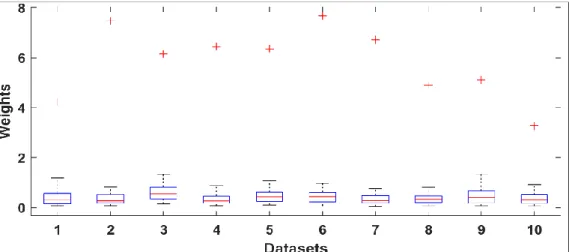
4.3 Results ... 35
4.3.1 Semi-Simulated EEG Dataset ... 35
4.3.2 Resting State EEG Dataset ... 40
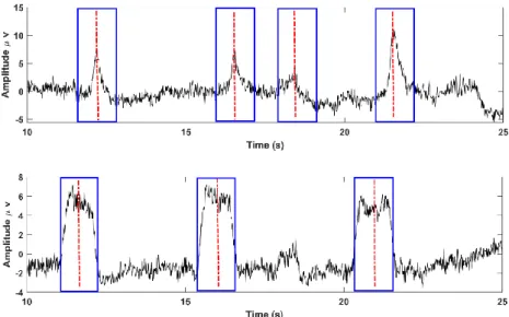
4.3.3 PhysioNet P300 ERP Dataset ... 42
4.4 Summary ... 45
5 REMOVAL OF CARDIAC ECG ARTIFACTS ... 46
5.1 Subject and Methods ... 46
5.1.1 Pre-processing ... 46
5.2 Datasets... 53
5.3 Results ... 53
5.3.1 Artifact Detection Performance Metrics ... 54
5.3.2 QRS Detector Performance ... 54
5.3.3 ECG Component Classifier Performance ... 56
5.4 Summary ... 56
6 FUNCTIONAL CONNECTIVITY IN ISCHEMIC STROKE ... 58
6.1 Overview of Connectivity Association Measures ... 59
6.1.1 Functional Connectivity Association Measures ... 59
6.1.2 Effective Connectivity Association Measures ... 61
6.2 Overview of Connectivity Network Metrics ... 63
6.3 Functional Connectivity Biomarkers for Monitoring Ischemic Stroke Recovery ... 65
6.3.1 Subject and Methods ... 67
6.4 Results ... 69
6.5 Summary ... 73
7 HIGH-RESOLUTION DYNAMIC FUNCTIONAL CONNECTIVITY ... 74
7.1 A Critique of the Sliding-Window Dynamic Connectivity ... 75
7.2 Dynamic Connectivity based on the Empirical Mode Decomposition ... 79
VII
7.3 Validation using Synthetic Signals ... 83
7.4 Validation using a Finger-tapping Experiment ... 87
7.5 Summary ... 93
8 CONCLUSIONS ... 95
9 SUMMARY OF THE MAIN CONTRIBUTIONS ... 97
9.1 Thesis I: Novel method for removing EOG artifacts ... 97
9.2 Thesis II: Novel method for removing ECG artifacts ... 97
9.3 Thesis III: Functional connectivity biomarkers for stroke monitoring ... 97
9.4 Thesis IV: New method to increase the temporal resolution of dynamic functional connectivity ... 97
LIST OF PUBLICATIONS ... I
REFERENCES ... I
1
1 Introduction
Electroencephalography (EEG) is a non-invasive method used to measure the bioelectric activity of the brain using electrodes placed on the scalp. The simplicity of the measurement and the high temporal resolution of the recorded signal make EEG essential e.g. in epilepsy diagnosis, cognitive or sensorimotor experiments, where rapid activity changes must be examined. The source of the activity is the change in the postsynaptic potentials of cortical neurons acting as tiny current generators placed in a direction perpendicular to the cortical surface. When a sufficiently large population of nearby neurons is activated simultaneously, the generated current fluctuations cause detectable changes in the electrical field of the brain [1].
The scalp potential distribution, generated by this electric field, can be measured by a suitable EEG measurement device and a set of scalp electrodes, and can be stored in a computer for later processing and analysis. The number and layout of the electrodes used in practice can vary greatly, but high-density 64 or 128-electrode systems arranged in the universal 10/10 or 10/5 layout [2] are the most common in research laboratories. The main advantage of EEG over other brain imaging methods (e.g. fMRI, PET) is its superior temporal resolution. Typical EEG sampling rates are in the range of 512 to 4096 Hz, which enable us to follow the time course of brain activity at millisecond or sub-millisecond resolution.
1.1 EEG Artifacts
The measured EEG signals are regularly contaminated by equipment and environmental noise as well as artifacts caused by extracerebral physiological sources. Among the latter types, ocular, muscle and cardiac artifacts are especially problematic due to their high amplitude and non- periodic (ocular, muscle) or quasi-periodic (cardiac) nature. Other kinds of artifacts generate physical noises that appear as power line noise or variations in electrode-skin conductivity.
Artifacts can easily turn valuable EEG measurements unusable. The quality of measured data can further reduce due to the presence of low-quality sensors (electrodes) or bad trials. A trial here refers to a data segment whose location in time is typically locked or related to certain experimental protocol. In other cases, in a task-free protocol such as resting state, a trial represent a data segment of certain length of time.
Ignoring the presence of low-quality data (a bad trial or bad sensor, etc..) can have an adverse effect on downstream performance of the desired experiment. For example, when averaging multiple trials time-locked to the stimulation to estimate an evoked response, a single bad trial can corrupt the final averaged EEG signal. Bad channels are also potential problems, as artifacts present on a single bad sensor can spread to other sensors due to spatial projection. Normal filtering techniques [3] can often suppress many low frequency artifacts, but turn out to be insufficient for broadband artifacts since the artifacts usually have frequencies overlapping with the signal frequency, which makes artifact removal a key step in every EEG processing pipeline.
Early attempts to remove ECG artifacts from EEG included subtraction and ensemble average subtraction (EAS) [4] methods. Current mainstream methods are based on adaptive filtering [5,6]
and blind source separation such as Independent Component Analysis (ICA) [7,8] which is
2
widely used in the field of EEG signal processing for artifacts suppression, since it can separate a signal mixture into its main sources, such as EOG, ECG, EEG, etc. components. Wavelet transform (WT) is increasingly used [9,10] in the EEG noise removal and it is more often used in combination with (ICA)-based methods [11,12].
The simplest method is to discard parts of the data that are contaminated by artifacts. This approach requires visual inspection and manual rejection of artifact contaminated data segments or epochs. This is a labour-intensive task that requires a trained expert to go through each individual dataset to mark artifacts, and it excludes the possibility of automatic and high-speed analysis of large-scale EEG experiments. Although the annotation of bad EEG data is likely to be accepted by trained experts, their decision is subject to variability and cannot be replicated.
Their assessment may also be skewed due to prior experience with specific experimental setup or equipment, not to mention the difficulty these experts have in allocating enough time to review the raw data collected daily.
Since visual inspection is slow, tiring and requires an expert assistant, several authors proposed methods for semi or fully automatic component detection, which resulted in automated analysis pipelines [13]. The automation approach not only saves time, but also allows flexible analysis and reduces the barriers to reanalysis of data, thus facilitating reproducibility. One semi- automated method using ICA for identifying artifact components is presented by Delorme et al.
in [14]. Various statistical measures (entropy, kurtosis, spatial kurtosis) are calculated for each independent component to label them automatically as artifact, but validation and rejection is performed manually. Since the method is based on statistical analysis of the components, which does not consider the physiological model of artifacts, the performance of the method is not perfect. A similar statistical approach is followed in the FASTER [15] and ADJUST [16] artifact removal toolboxes.
Brainstorm, EEGLAB, FieldTrip, MNE,[17–20] are popular tools used for rejection of EEG artifacts based on simple metrics such as differences in peak-to-peak signal amplitude that are compared to a manually set threshold value. When the peak-to-peak amplitude differences in the EEG exceeds a certain threshold, the given segment is considered bad that should be excluded from the experiment. Kurtosis, standard division, mean, skewness etc. are used to set the proper threshold and remove the peaks or trials greater than the threshold e.g. trial has kurtosis >5 is rejected. Although this seems to be very easy to understand and easy to use from the point of view of a practitioner, it is not always convenient. Moreover, a good peak-to-peak signal amplitude threshold is data-specific, meaning that setting it involves a certain amount of testing and error. Rejection of data epochs can result in significant loss of data which in turn can have adverse effects in Event Related Potential (ERP) studies. Using only a small number of remaining epochs can result in critically low signal-to-noise ratio.
More sophisticated artifact removal methods rely on cross-correlation based filtering which require the use of reference channels, in the form of e.g. horizontal-vertical eye movement (EOG) or ECG electrodes. These can be acceptable in strictly controlled laboratory situations, but extra electrodes can be problematic in clinical settings due to patient discomfort or interference with other equipment. Numerous researches have therefore been directed towards creating automatic artifact removal methods that work without external electrodes and can be performed without manual inspection. The most successful ones of such methods are based on the application of Independent Component Analysis (ICA) [8] that can separate a signal mixture into its original sources or components, based on the condition of statistical independence.
3
Bad channel artifacts generate high amplitude and non-periodic signal effects, which distort raw EEG data, making EEG calculations untrustworthy. Rejecting the trial which has drifts is not practical solution because if there is one bad channel displayed on the data, it means most of the trials would be rejected [21]. Consequently, only the bad channel has to be automatically marked and interpolated to avoid rejecting entire trials. The traditional artifact removal approach based on visual inspection has no standard measure from one to another about how we define and reject the artifacts. In the manual inspection protocol, the electrode offset has to be checked before starting the real experiment to mark the bad channels. The pre-defined information about the bad channel list needs to be updated if one of the channels contains bad records in the middle of the measurements, and this can be hard to detect during the recordings if no significant variance can be detected in the channels.
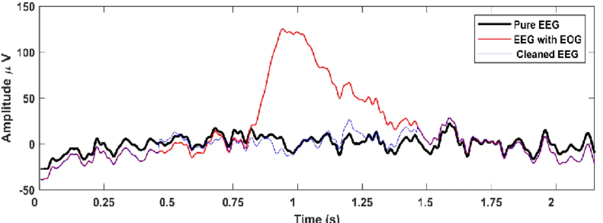
In this thesis, fully automatic methods for removing EOG and ECG artefacts from EEG signals are proposed. A new wavelet-based method is presented for EOG artifact removal that cleans EOG independent components selectively, leaving non-contaminated parts of the component untouched. The novel ECG artefact removal algorithm uses a sophisticated approach to identify automatically the ECG components without the need for a reference ECG channel, thus it can be used in situations where ECG data is not available. The method can also detect and remove ECG artefacts generated by pathological cardiac activities which makes the method more robust when analysing EEGs of elderly patient. The results show that the proposed methods outperform state- of-the-art methods for EOG-ECG removal in its accuracy both in the time and the spectral domain, which is considered an important step towards the development of accurate, reliable and automatic EEG artifact removal methods.
1.2 Brain Connectivity
The human brain comprises close to hundred billion neurons, each establishing several thousand synaptic connection matrices which can be mathematically modelled in several scales micro- meso-macro-scale levels, with nodes or regions and links. Connectivity refers to the anatomical connected patterns (networks pathways) of the nervous system ("anatomical connectivity"), which have statistical dependencies ("functional connectivity") or these patterns have causal interactions ("effective connectivity") between distinct regions within a nervous system. To go beyond these networks and decode the meaning of connectivity links between the nervous cells or regions is one of the goals of neuroimaging. Studying these links is crucial to elucidating the strength of connection and describing the direct and indirect information flow at different scales such as individual synaptic neurons at the microscale or pathways between regions at the macroscale. Properties of the connectivity network may help in deciding whether certain neural regions are normal or contain unexpected features caused by functional deficits or neuropsychiatric disorders.
Through identifying anatomical and functional associations of brain regions on the same map using an integrated approach, brain mapping techniques, network analysis becomes a powerful tool for investigating structural-functional mechanisms. It is able to present the brain connectivity and to reveal etiological relationships that link abnormalities of connectivity with neuropsychiatric disorders.
4
1.3 Brain Connectivity Biomarkers of Diseases
Ischemic stroke is one of the major causes of death or permanent disability with increasing frequency of occurrence as the population in developed countries is aging. Prompt and effective treatment can speed up recovery and improve rehabilitation outcome. Timely treatment of stroke starts with an MRI and/or CT scan to identify the location and extent of brain damage. After diagnosis, treatment starts and the condition of the patient is monitored by the medical staff based on external symptoms using standardized stroke scales (NIHSS, BI, etc.) [22,23]. A second MRI scan might be performed on patient dispatch to confirm recovery status. Unfortunately, complications can develop in the hospital, e.g. Delayed Cerebral Ischemia (DCI), which can only be discovered once symptoms worsen [24]. Also, efficiency of the treatment is difficult to assess without monitoring quantitative stroke metrics. These metrics could help in selecting the best treatment path, and be used as predictors for the level of recovery at the end of the rehabilitation period [25–28].
Continuous monitoring of patients and the use of mainly frequency-domain quantitative measures have already been suggested [28–31]. It is known that these metrics can detect stroke- related status changes well before symptoms develop [28]. The reported methods all rely on the calculation of a single metric from measurements using a standard 19-electrode clinical EEG system. This process could be more efficient with using high density electrode-cap of 128 or 256 channels with more metrics describing the properties in-between the different brain regions.
This thesis develops brain connectivity metrics based on high-density EEG measurements that can depict the location and extent of stroke lesions similar to MRI scans. Monitoring brain connectivity changes could help in verifying treatment effectiveness as well as measuring progress of recovery. A comparison of connectivity measures is performed between patients and control group as well as between start and end of the stroke rehabilitation interval. The results show differences in the small-world, graph degree, clustering coefficient, global and local efficiency metrics that correlate with brain plasticity changes during stroke recovery and can be used as biomarkers to quantify stroke severity and outcome of recovery.
1.4 High Resolution Brain Connectivity
Precise and accurate analysis of the non-stationary spectral variations in EEG is a long-standing problem. Dynamic Functional Connectivity (DFC) is an emerging subfield of functional brain connectivity analysis whose goal is to uncover and track the changes in functional connectivity over time. Traditional connectivity methods assumed that the connectivity network representing cortical activity is stationary. Dynamic connectivity can provide new insights about the large- scale neuronal communication in the brain and help to track the progress of recovery of many neurological disorders and brain diseases such as epilepsy, Alzheimer’s disease, stroke, and predict outcome to many other deficits related to the brain. The crucial part of calculating DFC is the time-frequency decomposition.
The Fast Fourier Transform (FFT) has been used to efficiently estimate the frequency content of a discrete and finite time series but it assumes the input signal is stationary. The most important issue in the time-frequency analysis of an EEG signal is the principle of uncertainty, which stipulates that one cannot locate a signal with an absolute precision both in time and frequency.
Over the past 30 years, several methods have been developed to extend Fourier's research to non- stationary signals, resulting in a body of work called "time-frequency" (TF) representation
5
methods. They include linear TF methods as Short Time Fourier Transform (STFT), Wavelet Transform (WT) that involve phase and magnitudes contributions.
The Short-time Fourier and the wavelet transforms also show some resolution limitations (localization limit) due to the trade-off between time and frequency localizations and smearing due to the finite size of their templates. STFT is the extension of FT which was modified to show nonstationary components of the signal in time. It is indeed the FFT of the successive, overlapped windows of the signal, where each frequency distribution is being correlated with each window's central time. Usually there is a peak smeared around the peak of the main frequency with decaying side lobes on the selected window. However, side lobes attenuation is associated with increasing of the window [32]. The spectral smearing can be reduced by increasing the length of the time window, but this also reduces the time localization accuracy by imposing increased stationarity. Thus, high time localization comes at the expense of the spectral smearing.
Wavelet transformation was established for the time varying spectral estimate to overcome the spectral smearing. It uses variable time window lengths which are inversely proportional to the frequency of the central target. So, long windows used for low frequencies therefore have good frequency, but limited time, while short windows used for high frequencies have good time but limited range of frequency resolution [33]. WT showed accepted temporal resolution on the high frequencies, while poor temporal resolution was located in the low frequencies [34]. The chosen wavelet function should be carefully selected with specific characteristics to improve the signal representation.
Functional connectivity emerging from phase synchronization of neural oscillations of different brain regions provides a powerful tool for investigations. While the brain manifests highly dynamic activation patterns, most connectivity work is based on the assumption of signal stationarity. One of the underlying reasons is the problem of obtaining high temporal and spectral resolution at the same time. Dynamic brain connectivity seeks to uncover the dynamism of brain connectivity, but the common sliding window methods provide poor temporal resolution, not detailed enough for studying fast cognitive tasks. In this work, I propose the use of the Complete Ensemble Empirical Mode Decomposition (CEEMD) followed by Hilbert transformation to extract instantaneous frequency and phase information, based on which phase synchronization functional connectivity between EEG signals can be calculated and detected in every time step of the measurement. The work demonstrates the suboptimal performance of the sliding window connectivity method and shows that the instantaneous phase-based technique is superior to it, capable of tracking changes of connectivity graphs at millisecond steps and detecting the exact time of the activity changes within a few milliseconds margin. The results can open up new opportunities in investigating neurodegenerative diseases, brain plasticity after stroke and understanding the execution of cognitive tasks.
1.5 Thesis Organization
This section describes the structure of the thesis, starting from Chapter 2 which presents an introduction to the characteristics of EEG, the measurement process and required equipment, and the steps to record an acceptable EEG measurement. Then, it gives an overview about the pre- processing approaches used in EEG signal processing.
6
Chapter 3 starts with defining the different types of EEG artifacts, which can be formed by biological or external sources, followed by an overview of the state-of-the-art techniques for EEG artifacts removal.
In Chapter 4, I provide an improved, fully automatic ICA and wavelet based EOG artifact removal method that cleans EOG independent components selectively, leaving other parts of the component almost untouched.
A novel automatic method for cardiac artifact removal from EEG is discussed in Chapter 5.
Both proposed methods work without manual intervention (visual inspection), and thus accelerates pre-processing steps and lay the groundwork for potential online and real-time EEG analysis (e.g. BCI and task related application, finger tapping, visual - auditory evoked potentials).
A high-resolution EEG technology as an aid for monitoring and quantifying patient recovery progress, complementing the use of clinical stroke scales is introduced in the first part of Chapter 6. Connectivity network metrics are calculated as an aid for monitoring and quantifying patient recovery progress, complementing the use of clinical stroke scales. It shows changes of functional connectivity measures in stroke patients to identify reliable biomarkers that characterize progress of recovery and predict outcome. To overcome the trade-off between time and frequency resolution and localization smearing, in Chapter 7, I propose the use of the Complete Ensemble Empirical Mode (EEMD) Decomposition followed by Hilbert transformation to extract instantaneous frequency and phase information. The results showed that the introduced method is able to track the fast-dynamic brain connectivity changes in time and frequency resolution at rate of sampling frequency.
Finally, in Chapters 8 and 9, I conclude the results of the thesis work and list my publications related to the presented work.
7
2 Introduction to EEG signal Processing
I start this chapter with discussing the characteristics of EEG data, the process of EEG measurements, the equipment needs for the measurement, and the steps to record an accepted EEG measurement. Then, I give an overview of the pre-processing approaches used with EEG measurements, the extracted features used to show the characteristics of the measured signal in the time and frequency domain and the concept of source localization and brain connectivity and their impact for neuroimaging sciences.
The history of EEG started around the end of the 19th century when an English researcher, Richard Caton (1842–1926) was able to detect electrical impulses of the brain using the exposed cortex of monkeys and rabbits [35]. He used a sensitive galvanometer to detect the fluctuations of the brain in different stages, sleep and absence of activity following death. Adolf Beck, (1863- 1939), a Polish physiologist did similar measurements, followed by Russian physiologist Pravdich-Neminski (1879-1952) who presented a photographic record. The German psychiatrist Hans Berger [36], in 1924, was the first researcher who recorded EEG measurements from a human. This led to measurements on epileptic patients (Fisher and Lowenback, 1934). Gibbs, Davis, and Lennox [37] in 1935 described interictal epileptiform discharge wave patterns during clinical seizures. The English physician Walter Grey in the 1950's developed EEG tomography which provided a means for mapping electrical activity across the surface of the brain. It gained its prominence during the 80's primarily as an imaging technique in research settings.
2.1 Overview of the Measurement Process
The measured EEG signal is the sum of all the synchronous activity of all cortical sources including areas potentially far away from a given electrode. The scalp potential distribution, generated by this electric field, can be measured by a suitable EEG measurement device and a set of scalp electrodes, and can be stored in a computer for later processing and analysis. The recording system consists of electrodes, amplifiers with filters, A/D converter and recording device. Electrodes are used to record the signal from the head surface, then the recorded signals are fed into amplifiers. The signals are converted from analogue to digital form, and finally, a computer displays and stores the obtained data.
Electrodes EEG Instrument (A/D box) Graphical output Figure 2-1:Main components of an EEG measurement system1.
There are different types of electrodes, reusable disc electrodes, electrode caps, needle electrodes and saline-based electrodes. Each one of it has its own function; for example needle electrodes
1image source: https://www.biosemi.com/.
8
are used invasively where they are inserted under the scalp for long recordings while electrodes cap are preferred for multichannel montages, where they are installed non-invasively on the scalp surface. Commonly, scalp electrodes consist of Ag-AgCl disks, of diameter between 1 to 3 mm, and long flexible leads are plugged into an amplifier. The number of electrodes used in practice varies. In clinical practice, 19 electrodes are used. In research experiments, 32 to 256 electrodes may be used. There are several electrode layouts in use, such as the 10/20, 10/10 or 10/5 international systems, or the Biosemi ABC radial layout [2] as shown in Figure 2-2 and Figure 2-3 . The channel configurations can comprise up to 64 -128 or 256 active electrodes.
Figure 2-2: The international 10-20 electrode layout.
Figure 2-3: Biosemi cap, 128-channel ABC radial layout.
The main advantage of EEG over other brain imaging methods (e.g. fMRI, PET) is its superior temporal resolution. Typical EEG sampling rates are in the range of 512 to 4096 Hz, which enable us to follow the time course of brain activity at millisecond or sub-millisecond resolution. The head is made up of various tissues (white and grey matter, cerebrospinal fluid, skull, scalp) with varying conductivity properties. When the generated current flows from the cortex to the scalp, it must pass through the skull which has a relatively low conductivity (high resistivity). As a result, the current spreads out laterally within the skull instead of passing straight through to the scalp. The result of this so-called volume conduction effect is the reduced spatial resolution and
9
the ‘smeared’ or ‘blurred’ appearance of activation sources on the scalp potential distribution image.
EEG is widely used in many applications as part of diagnosis and monitoring of epilepsy [38], Parkinson's disease [39], Alzheimer’s disease [40], Huntington's disease [41], events detection in healthy human sleep EEG [42], brain-computer interface (BCI) [43] and can help in the localisation of the exact cortical source of the activity or disease [44].
2.2 EEG Processing Pipeline
EEG data is normally processed in a pipeline fashion, starting with data pre-processing including filtering, artifact removal, re-referencing, followed by feature extraction (Event-Related Potential, time-frequency, cortical source or connectivity features) followed by classification or pattern recognition.
Figure 2-4: EEG processing pipeline 2.2.1 Pre-processing
One of the most critical steps to obtain a clean EEG data is the pre-processing phase. Noise, unwanted artifacts, and other disturbances must be removed from the signal in order to produce reliable results. The EEG signal can contain physiological and non-physiological noise and artifacts, e.g. effects of eye and body movements, muscle contraction induced noise, heart and pulse artifacts, superimposed mains power line noise of 50 or 60 Hz and its harmonics, and amplitude variations by changes at the tissue/electrodes interface (due to skin resistance variation or contact problems).
Bandpass/band stop filtering is one of the classical and simple attempts to remove artifacts from an observed EEG signal. This method works reliably only when the artifacts have a narrow frequency band, e.g. power line artifact (50/60 Hz, see Figure 3-1), and the spectrum of the artifacts do not overlap with the signal frequency. Band pass filtering from 0.1 to 70 Hz is used to initially to keep only the meaningful frequency range of the EEG signal. However, in some cases, fixed-gain filtering is not working efficiently for biological artifacts because it will attenuate EEG interesting signal and change both amplitude and phase of signal [45]. Adaptive filtering [46] is an alternative approach to the normal filtering method, which assumes that the EEG and the artifacts are uncorrelated, and the filter parameters are adjusted in a feedback loop.
Adaptive filtering, however, requires a reference signal for correct operation.
Wiener filtering is considered also an optimal filtering technique used as the adaptive filtering.
It uses a linear statistical filtering technique to estimate the true EEG data with the purpose to create a linear time invariant filter to minimize the mean square error between the EEG data and the estimated signal [47]. Since there is no a priori knowledge on the statistics [48], the linear filter estimates the power spectral densities of the observed signal and the artifact signal, moreover it eliminates the limitation of using extra reference channels, but the requirement of calibration can add the complexity of its application.
EEG data Pre-processing Feature
Extraction
Classification/
Pattern recognition
10
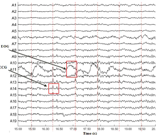
Figure 2-5: EEG raw data contaminated with EOG and ECG artifacts.
Since the electrical potential of the physiological artifacts have frequency characteristics overlapping with the EEG signal, the removal of such kind of artifacts needs more efficient methods since the traditional signal processing techniques such as normal filtering method fail to clean them. Researchers have developed different methods for artifact removal, including adaptive filtering and component-based method. In the adaptive filtering-based method, a recursive algorithm is used for updating filter coefficients. The coefficients are modified until the output has been minimized according to a given signal property (e.g. time and frequency domain features) to remove the noises out of the signal [45]. Thus, a reference signal, has to supplied besides the recorded signal (Figure 2-6).
11
Figure 2-6: Overview of the adaptive signal filtering method [46].
Independent Component Analysis (ICA) is one of the component-based approaches that are commonly used in the pattern analysis and biosignal analysis [49]. ICA is able to separate the artifacts from the signals by decomposing the EEG signals into several independent components based on statistical independence of signals. One of the main advantages of this method that it does not need an external reference channel, as the algorithm itself does not need a priori information. Once the signal is decomposed into independent components, one or more components will represent the artifacts. If these components are removed before reconstructing the signal from the components, we will get an artifact-free signal. There are two methods for identifying and removing artifact components, i) manual visual inspection where an expert searches for the bad component to reject, and ii) automatic detection where the component is compared with a pre-defined threshold [15,50]. The manual component inspection is time consuming and cumbersome. Automatic component detection depends on passing the signal to a sophisticated algorithm using the pre-defined threshold or reference channels to help in identifying artifact components. The details of each method are described in the Chapter 3.
2.2.2 Feature Extraction
After artifact removal, the significant features of the cleaned EEG signals will be extracted by using feature selection methods. The feature extraction and selection methods are important to identify certain properties to be used effectively in classifying the EEG signals. In addition, it also reduces the amount of resources needed to describe a huge set of data accurately. Hence, feature extraction is considered the most critically significant step in EEG data classification.
Several methods are used in feature extraction including time-domain, frequency domain and time-frequency domain. In the time-domain, the commonly used features are, mean, minimum, maximum, variance, entropy, etc. The drawback of the time-domain approach is its high sensitivity to variations of the signal amplitude.
12
In the frequency domain, the signal is transformed into frequency domain using Fast Fourier Transform (FFT). Frequency characteristics are dependent on neuronal activity and grouped into multiple bands (delta:1-4 Hz, theta:4-8 Hz, alpha:8-12 Hz, beta:12-30 Hz, and gamma :>30 Hz) corresponding to a cognitive process. In some cases, frequency characteristics are not enough to provide signal characteristic for classification using only frequency information, which makes the time-frequency domain the alternative to improve the classification performance [51]. These include wavelet transform (WT) which is highly effective for non-stationary EEG signals compared to the short-time Fourier transformation (STFT). Several feature extraction methods have been used based on the time-frequency domain approaches as Power Spectrum Density, Phase Values Signal Energy. Calculating the coherence between the different time-frequency signals refers to an important feature called connectivity. These connectivity features include Magnitude Squared Coherence, Phase Synchronization, Phase Locked Value, etc. The most important issue in the time-frequency analysis of the EEG signal is the principle of uncertainty, which stipulates that one cannot localize a signal with absolute precision both in time and frequency. This principle controls the time-frequency characteristics and is considered as a cornerstone in the interpretation of Dynamic Functional Connectivity (DFC).
2.2.2.1 Event Related Potential (ERP) computation
The amplitude of the EEG signal measured on the scalp is normally within the range of ± 50 μV.
The biologically meaningful small-amplitude signal is usually embedded in relatively high level of noise generated by various biophysical sources (muscle activity, ECG, eye movement, blinks), skin resistance changes, electrode malfunction, and so on, making the detection of small amplitude changes difficult. A well-established method for this problem is signal averaging.
Assuming that noise is a random process with zero mean, the sample-wise averaging of a sufficiently large number (>100) of EEG trials (time window of task of interest) in a stimulus- synchronised manner will cancel out noise and leave only the stimulus-locked components in the resulting signal [52]. Successful averaging requires very precise synchronisation of the datasets of the repeated experiments; therefore, stimulus presentation and response triggers are used to mark the start and end of the experiment trials. Depending on which trigger is used for averaging, we can distinguish between stimulus or response-locked averaging. The resulting trigger-based average potentials are called event related potentials (ERP). Depending on the applied stimulus type, we can examine visual, auditory, sensory and other cognitive tasks with this method.
The execution of cognitive tasks involves various sensory, cognitive and motor processes. The sum of these processes appears in the averaged ERP waveforms in the form of components.
Components are distinct positive or negative potential peaks, as illustrated in Figure 2-7, named by the polarity (negative/positive) and the order or time stamp of the peak, e.g. N1, N2, P1, etc.
or N100, P300 or P500. The analysis of these waveforms allows us to compare ERPs obtained under different conditions and consequently test scientific hypotheses.
13
Figure 2-7: Typical ERP components: positive and negative peaks designated by their order P1, P2, P3 or the time they appear, e.g. P100, N400. ERP is often displayed with reversed polarity showing negative peaks pointing upwards. (Source: https://en.wikipedia.org/wiki/ Event-related
potential).
2.2.2.2 EEG Source Localization and Connectivity
EEG source localization can be used to uncover the location of the dominant sources of the brain activity using scalp EEG recordings. It provides useful information for study of brain's physiological, mental and functional abnormalities by solving inverse problem. The process involves the prediction of scalp potentials from the current sources in the brain (forward solution) and the estimation of the location of the sources from scalp potential measurements (termed as inverse solution) [53]. The accurate source localization is highly dependent on the electric forward solution which includes, head model, the geometry and the conductivity distribution of the model tissue sections (scalp, skull, brain grey, cerebrospinal fluid, and white matter, etc.).
In EEG connectivity analysis, methods based spectral coherence such as Phase Lock Value, Phase Lock Index, etc. [54] replace amplitude correlation to mitigate the effect of noise and reduce spurious connections caused by volume conduction. Connectivity can be computed in the sensor (electrodes) space or in the source (cortex) space. Connectivity in source level requires accurate 3D head models and sophisticated inverse problem solvers needs it also requires a lot of complicated work includes first doing forward solution which needs information about the anatomical structural of the brain as:
• Head model which contains the voxels and the connectivity of the brain layers.
• Source model: which contains the information about the dipole’s positions and orientations.
The above steps need information about the anatomical data and anatomical marks to align the sensors with the anatomical marks before starting source reconstruction. Preparing the head model dependent on the used method for preparing the volume conduction such as Boundary Element Method (BEM) and Finite Element Method (FEM). BEM calculates the model on the boundary of the head (scalp, skull, brain), while FEM calculates the model on all points of the head. The calculation of the connectivity is slow due to many arguments need to be defined. The increasing in the source depth deteriorates the accuracy of the connectivity estimations due to the decreased accuracy of source localization and size. A problem of source reconstruction in EEG is that the sources may not be fully spatially determined, but rather are smeared out across a
14
relatively large brain volume. This problem arises mainly from inaccurate forward solution and the ill-posed nature of the inverse EEG problem, which projects data from relatively few electrodes to many possible source locations. This might result in two uncorrelated sources having their reconstructed time courses erroneously correlated. Ignoring this can artificially inflate the level of connectivity between two sources. The way leakage propagates across the source space is non-trivial, and solutions are required to be implemented to decrease this effect on functional connectivity [55]. Since connectivity in the source space cannot be calculated without the anatomical information of the brain, calculating connectivity in sensor space is a much faster approach, however, with reduced spatial resolution.
2.3 Current State-of-the-Art Methods
Event-related and time-frequency analysis methods can be used to verify hypothesis based on various experimental conditions and to explore the temporal/spectral/spatial characteristics of the EEG data. Time-frequency analysis methods provide a more advanced set of tools that provide information of activity in different frequency bands and lend themselves naturally to the examination of oscillations and phase properties of the given cognitive process. It allows us to better separate the components of a task that contain perceptual, cognitive and decision subtasks.
Time-frequency analysis results also more naturally connect with neural mechanisms at lower spatial scales. They do not, however, provide information about the nature and operation mechanisms of the distributed cortical networks underlying the given cognitive processes. On the other hand, finding the correlation between the calculated frequency characteristics give a clear insight where understanding brain function involves not only gathering information from active brain regions but also studying functional interactions among neural assemblies which are distributed across different brain regions. This frequency correlation is well known as brain connectivity and widely used to aid diagnosis of neural and brain diseases such as stroke, Alzheimer’s disease, epilepsy, etc. It provides important biomarkers for understanding pathological underpinnings, in terms of the topological structure and connection strength and opens the way to the network analysis which has become an increasingly useful method for understanding the cerebral working mechanism and mining sensitive biomarkers for neural or mental problems as language processing [56,57].
Connectivity analysis, the collections of methods for investigating the interconnection of different areas of the brain – provides the theoretical basis as well as the practical tools describing the operation of these networks [58]. Different areas of the brain are connected by neural fibres or tracts of the white matter, transmitting information between distant brain regions. This type of connectivity, the Structural Connectivity, describes the anatomical connections in the brain.
Diffusion Tensor Imaging [59] can be used to detect anatomical fibres and construct structural networks. Structural connectivity, however, presents a rather static and limited view of the brain;
it cannot fully describe the short-range, dynamic and plastic interconnection and activation mechanisms found in brain processes. Functional and Effective Connectivity networks provide this crucial additional information for us [60]. Functional Connectivity describes the temporal correlations in activity between pairs of brain regions. The connectivity may reflect linear or nonlinear interactions, but it ignores the direction of the connection. Effective Connectivity, on the other hand, uses measures that enable it to describe causal influences of one region on another, hence explore dependencies in our network.
15
Figure 2-8: Varying information content extracted by different connectivity analysis methods2. Connectivity is described by networks, which are in fact graphs, consisting of nodes (brain regions) and edges (connections) [61]. Nodes ideally should represent coherent structural or functional brain regions without spatial overlap, while links represent anatomical, functional, or effective connections (link type) but can also have weight and direction associated with them.
Binary links only represent the presence or absence of a connection. Weighted links, on the other hand, can represent various properties. In anatomical networks, weights may represent the size, density, or coherence of anatomical tracts, while weights in functional and effective networks may represent respective magnitudes of correlational or causal interactions. In functional and effective connectivity networks, links with low weights may represent spurious connections that obscure the topology of strong connections. These can be filtered out using suitable thresholding policies.
To use these constructed networks in a quantitative manner, network measures/metrics are needed [61]. Measures can characterise the properties of local or global connections in the network, detect various aspects of functional integration and segregation, or quantify importance of individual brain regions. Measures exist at the individual element level or globally as distributions of individual measures. The degree of a node is the number of its links, i.e. the number of its neighbours, representing the importance of a node. The degrees of all nodes create a degree distribution which is important to describe e.g. the resilience of the network. The mean of this distribution gives the density of the network. Other measures, e.g. the number of triangles in the network, or the number of triangles around a given node (clustering coefficient) describe the level of functional segregation – the presence of functional groups/clusters – in the network.
Path length and average shortest path length provide information about the ability of the network to combine information quickly from distant brain regions. Further specific measures can be found in [61].
2image source: http://www.scholarpedia.org/article/Brain_connectivity
16
3 Literature review of EEG artifacts and possible removal
This chapter starts with defining the different types of EEG artifacts, which can be formed by biological and external sources, then it gives an overview of the state-of-the-art used techniques for EEG artifacts removal. Since the measured EEG signals are regularly contaminated by ocular EOG, and cardiac artifacts (ECG) that are especially problematic due to their high amplitude and non-periodic (ocular) or quasi-periodic (cardiac) nature, they can easily turn valuable EEG measurements unusable. Thus, I focus here on the state-of-the-art used techniques for removing the EOG-ECG artifacts from the EEG signal.
3.1 Noise and Artifacts
The measured EEG signals are regularly contaminated by equipment and environmental noise.
These noises vary between physiological or non- physiological sources. The non-physiological sources are represented by power-line noise, bad location of electrodes, unclean scalp, varying impedance of electrodes over the head, etc. as shown in Figure 3-1and Figure 3-2.
Figure 3-1: 60 Hz power line noise on channel 8 (affecting channels 1-7) and EOG artifacts (red highlight) spread over channels 1 to 7 (PhysioNet dataset- s01 rc02) [62,63].
17
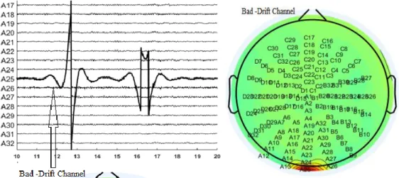
Figure 3-2: Illustration of a bad channel in a recording (electrode A25: potential drift, left panel) and its appearance in the scalp potential distribution (red spot in
the topoplot on the right panel).
The second kind of artifacts caused by extracerebral physiological sources such as ocular, muscle and cardiac artifacts that are especially problematic due to their high amplitude. The artifacts are either non-periodic (ocular- vertical or horizontal eyes movements, muscle) or quasi-periodic (cardiac) nature that can easily turn valuable EEG measurements unusable. Eye blinks - eye movements are the most common artifacts in EEG recordings. Eye movement generates changes in the resting potential of the retina during eye- movements and eye- blinks, besides the muscle activities of the eyelid within blinks produces disturbances in EEG recordings. The amplitude of EOG is generally much greater than the EEG and its frequency spectrum overlaps that of the EEG signals. They are mainly presented in low frequency components of the EEG, that is in between 2-10 Hz.
Figure 3-3: EOG physiological artifacts (horizontal and vertical eye movements) in the independent component (IC) space and their typical frontal high-amplitude pattern.
The heart also generates an electrical signal which can be recorded in numerous locations on the body, including the head which is called electrocardiograph (ECG) and has frequency band 0.5 - 100 Hz that overlaps with the EEG frequency [64]. Also, the heart during beating produces
18
artifacts that stem form voltage changes as blood vessels contract and and expand. This also generates low frequency components in the range of 0.5-3Hz affecting the characterization of K- complexes observed during stage N2 of NREM sleep and deep or slow-wave sleep (stage N3 of NREM).
Figure 3-4: ECG physiological artifacts in the ICs space and the scalp potential distribution of the QRS peak. Note the superimposed high-amplitude area in the left-occipital region.
The muscle artifacts from face, neck, and jaw generate an electrical activity called electromyography (EMG) that has high impact on EEG quality [64]. When jaw muscles are activated (teeth clenching and chewing) or if the head moves that involve neck muscle contractions, high amplitudes (in the order of mV) can be observed on the EEG measurements in the 20-30 Hz frequency range. Because head muscle activations are an inherent part of normal daily routines, solutions are needed that handle such artifacts. ICA might be considered an appropriate method to remove EMG contamination since both EMG contamination and EEG have substantial statistical independence from each other both temporally and spatially [65,66].
Changes in the quality of the electrical contact of channels over the skin produce the largest disturbance in the EEG. These kinds of artifacts are called motion artifacts, which influence the contact surface size, introduce skin deformation, and cause changes to the interface layer due to changes in conductive gel thickness or amount of sweat, resulting in electrical impedance change in turn. Artifacts of movement produced during normal activity, including locomotion, may have amplitudes greater than the signals produced by brain activity.
19
Figure 3-5: (a) Superposition of the true EEG signal (red) and the contaminating artifacts (blue). (b) Zoomed in view of the second contaminated signal section [67].
Unlike the artifacts mentioned above, which usually show stereotypical behaviour, movement or motion artifacts are non-stationary electrical signals. This makes cleaning of such artifacts one of EEG's major challenges. While the automated reduction of the artifacts has made substantial progress, there are only a few approaches that provide fully automatic artifacts handling methods for physiological artifacts [68].
3.2 Artifact Removal Methods
Artifact removal is a process of recognizing artifact components in the EEG signal and separating them from the neuronal sources. These strategies may use only EEG signals during artifacts rejection but may also rely on information from sources capturing physiological signals such as EOG, ECG, EMG. Most artifact rejection methods assume that the recorded signal is a combination of the signal of interest and the artifact signal, and the combination is additive in nature. Based on this fact, methods that are applied for artifact removal include regression, blind source separation (BSS : ICA and PCA), empirical mode decomposition (EMD), and wavelet transforms (WT) and in some cases, a combination of these methods is used [69,70].
A review of the most common EEG artefacts removal methods [71] provides a chart about percentage of the number of papers in the literature over the past five years (2015-2019), shown in Figure 3-6. It shows that Independent Component Analysis is the most frequently used method, moreover it was introduced with regression, WT, etc. as known as hybrid method to enhance the performance. Although there was an extensive research centred on artifact detection and removal of EEG signals reported in many literatures to date, there is no consensus on an optimal solution for all forms of artifacts, and the topic is still an open research problem [71].
20
Figure 3-6: Percentage of the number of literatures published during the past five years [71].
Visual inspection is one of the traditional methods used to remove artifacts; artifact contaminated or bad channel data segments (epochs) are simply rejected. This approach is laborious and can potentially lose useful neural information. Epoch rejection can largely reduce the number of usable epochs and reduce the signal-to-noise ratio. Manual inspection prevents the automatic and high-speed analysis of large-scale EEG experiments. The ICA-based source separation methods [72] could help in bad channel detection too, since bad channels show up as easily identifiable components as illustrated in Figure 3-7.
Figure 3-7: Bad channels (A25, D31) detected in the independent component space.
Spatial correlation with the other channels can be used to identify the bad channels [16,73,74]
but if correlation is low, these algorithms cannot identify the bad channel correctly. The correlation is mainly dependent on the distance between the electrodes: two distant electrodes might show low correlation although they might be phase-correlated. Automatic selection criteria based on statistical features are used in the FASTER [15] and EEGLAB [75]packages using pre- defined threshold such as z-score [15,18], which is still not robust since not all bad channel features can be described by the implemented features.
The DETECT package [50] is a MATLAB toolbox for detecting irregular event time intervals by training a model on multiple classes. The method showed results close to what they manually
21
identified, but is still dependent on the supervised learning method. An automatic bad intracranial EEG (iEEG) recordings was introduced by Viat et al, [74], using machine learning algorithm of seven signal features. The machine learning algorithm is supervised learning dependent and needs a large number of datasets and a variety of conditions for the training session. Correlation, variance, gradient, etc., were used as marker features identifying the deviation between the channels, however the method is dependent on supplying seven features to the trained network.
This implies that the data has to be pre-recorded to extract the features from the raw data, and consequently lose the real-time processing.
More sophisticated artifact removal methods rely on cross-correlation based filtering that require the use of so-called reference channels that record horizontal, vertical eye movements (EOG) and ECG activity. The use of reference electrodes can be acceptable in strictly controlled laboratory situations, but they can be problematic in clinical settings due to patient discomfort or movement.
3.2.1 Independent Component Analysis
Independent Component Analysis (ICA) [72] was originally developed for solving the Blind Source Separation (BSS) problem, which is considered a robust method for artifact removal able to minimize the mutual information between the different sources. ICA decomposes the EEG signals into independent components assuming that the sources are instantaneous linear mixtures of cerebral and artifactual sources. The two main approaches for measuring the independent sources are: minimization of mutual information and maximization of non-Gaussianity. The mutual information approach, informs how much information about the variable X could be gained from the information about the variable Y. The smaller value of mutual information means that more information about a given system is stored in the variables [76], so ICA algorithms based on mutual information approach are used to minimize the mutual information of the system outputs [19]. In the maximization approach, the algorithm has to modify the components in such a way to obtain the source signals of high non-Gaussian distribution (using the fact that: the stronger the non-Gaussian, the stronger the independence [76]). Different kind of metrics are used for maximization calculation as kurtosis, entropy, negentropy, approximations of negentropy and others [72].
Since ICA has unsupervised learning characteristics and works without a priori information and extra reference channels, it is used widely in the field of EEG noise (such as ECG and EOG artifacts) [11,21,70,77,78] removal. After source separation, estimated sources have to be identified as neuronal or artifactual sources to reconstruct the artifact-free EEG matrix where the unwanted artifacts (components) can be rejected by visual or automatic inspections.
Figure 3-8: Independent component analysis.